Diagnostic equipment

MT Pro

Diagnostic complex

Manual

Copyright © 2009-2010 MLab. All rights reserved Version dated 06/03/2010

Content

1. Introduction 4
   1. Purpose 4
   2. Opportunities 5
   3. System requirements. 6
   4. Specifications 7
2. Scope of delivery 10
3. Safety eleven
4. Preparation for work thirteen
   1. Installing the software. thirteen
   2. Installing the device driver. thirteen
   3. Preparing a PC to work with MT Pro thirteen
   4. Connection 14
   5. Grounding schemes. sixteen
5. Interface eighteen
6. Window management. twenty
7. Main menu 25
   1. Data export 26
8. Interface elements 31
   1. Graph Controls 32
      1. Moving the boundaries of the vertical axis. 33
      2. Changing the Scale of the Vertical Axis 35
      3. Offset / zero shift of the vertical axis 37
      4. Graphs and axes setup menu 39
      5. Group setting of the same type of parameters. 41
      6. Action groups with graphs / axes 42
   2. Parameter blocks 42
      1. Axis name block and graph 44
      2. Signal parameter block 45
      3. Block of parameters of markers 46
   3. Horizontal axis 47
      1. Changing the Scale of the Horizontal Axis. 47
      2. Navigation Along the Horizontal Axis 50
      3. Viewing a Signal While Recording 50
      4. Frame control panel 51
   4. Selected area 52
   5. Vertical and horizontal markers 53
   6. Pop-up menu of the home screen. 54
   7. Customizing Home Screen Items. 56
   8. Ruler 59
      1. Ruler setup 61
   9. Buttons with drop-down menu 63
   10. Control knob. 64
9. Oscilloscope 65
   1. Basic provisions 65
      1. Sampling frequency 65
      2. Channel input range 68
      3. Scan. 69

Content

• • 1. Synchronization 72
    2. Synchronization types 73
    3. Synchronization conditions 75
    4. Registration Modes. 76
  1. Oscilloscope window interface 78
     1. Toolbar 79
     2. Channel settings panel 80
     3. Channel control panel 82
     4. Sweep panel 83
     5. Synchronization panel. 84
     6. Marker position panel 85
     7. Control Panel 87
  2. Analog channel settings 88
     1. Analog channel settings list editing window 89
  3. Logical channel settings 94
     1. Window for editing the list of logical channels settings 96
     2. Setting the Logic Channel as the Label of the First Cylinder 99
  4. Work environment settings 101
     1. The window for editing the list of settings for the working environment 102

Introduction

This Operation Manual (OM) is intended to familiarize you with the basic rules of operation of the MT Pro diagnostic complex, as well as the software (SW) supplied with the equipment. Please read the contents of this manual carefully before using the instrument.

Purpose

The MT Pro diagnostic complex is designed for in-place diagnostics of automotive internal combustion engines, including the ignition, fuel supply, gas distribution, power supply systems, etc., reading information from the electronic control units (ECU) of the car using the OBD II protocol (for the version of the device with built-in OBD II scanner). MT Pro is a universal measuring device that is not tied to any particular brand or model of car, i.e. allows you to diagnose all makes and models. The device almost always provides the ability to directly connect sensors and probes to the corresponding electrical circuits of the car, without the need for additional adapters, dividers, etc.

Opportunities

Opportunities

The MT Pro diagnostic complex allows you to effectively detect a malfunction in the following systems:

Ignition system

§ Determination of the condition of spark plugs and spark plug wires (carbon deposits, breaks, breakdowns)

§ Determination of operating modes and malfunctions of the ignition coil (inter-turn short circuits, control of correct connection, breakdowns)

§ Diagnostics of sensors of the ignition system (inductive, hall)

§ Determining the ignition timing (without stroboscope)

Fuel supply system

§ Electrical check of fuel injectors (turn-to-turn short circuits of the injector windings, duration of the injection phase, etc.)

§ Checking the operation of temperature sensors, throttle position, oxygen sensor, mass air flow sensor, etc.

§ Checking the operation of actuators (idle speed controller, etc.)

Gas distribution system §

Assessment of relative compression by cylinders in the starter cranking mode Compression

§ measurement in dynamics (with the engine running) and in cranking mode Determination of

§ the correct installation of the timing belt

§ Valve control

Power and Charging System

§ Checking the operation of the generator and the battery charging system

With a built-in OBD II scanner, it allows you to perform §

Vehicle identification Reading and deciphering fault codes Resetting

§ stored information about fault codes Displaying the status of sensors

§ in digital and graphical form

§

§ Display of the system status (freeze frame) at the time of the malfunction Reading and

§ interpretation of the results of the oxygen sensor test

§ Actuator control

Functionality §

Simultaneous display on the screen of data from 1,2, 3 … 7, 8 analog channels and 1 logical channel

§ Possibility of synchronization from the signals of almost all electrical circuits of the car Long signal

§ acquisition time (limited by available disk space) Possibility to save data on received signals and support

§ reports

System requirements

System requirements

Minimum

§ Operating system: Windows 98 / ME / 2000 / XP / Vista (under development)

§ Processor: Celeron / Pentium II 600 MHz

§ RAM: 64 MB (Win98 / ME) / 128 MB (Win2000 / XP) Available disk

§ space: 128 MB

§ Hard disk controller: support for DMA transfer mode Video

§ adapter: 800×600, 256 colors

§ USB interface: 1.1

Featured

§ Operating system:Windows XP SP2 § Processor:Pentium III 1 GHz or better §

RAM: 256 – 512 MB

§ Available disk space: 1 – 2 GB Hard disk controller: DMA transfer

§ mode supported Video adapter: 1024 x 768 True Color

§

§ USB interface: 2.0

Specifications

Analog channels

§ Number of universal analog channels: Number of

§ simultaneously switched on channels:

§ Channel input range:

§ Channel subranges:

§ Number of subbands of the channel: Input

§ active impedance of the channel:

eight

in oscilloscope mode: 1, 2, 4 or 8 in

recorder mode: 1, 2, 3, 4, 5, 6, 7, 8 ±1000 V

±2, ±5, ±16, ±30, ±80, ±200, ±500 and ±1000 V 8

not less than 1 MΩ

Logical channelsone)

§ Number of universal logical channels: Number of

§ simultaneously enabled channels: Channel input

§ range:

§ Channel subranges:

§ Number of subranges of the channel: DAC bit depth

§ for setting the comparison threshold: Input active

§ resistance of the channel: Optionally connected pulse

§ detector:

one

1 (visible only in recorder mode) ±1000 V

±2, ±5, ±16, ±30, ±80, ±200, ±500 and ±1000 V 8

12 bit

not less than 1 MΩ

Yes

Maximum sample rate2)

§ In oscilloscope mode: 2 MHz (in 1-channel mode) 1 MHz (in 2-channel mode) 250 kHz (in 4- channel mode) 125 kHz (in 8-channel mode)

§ In recorder mode: 500 kHz (in 1-channel mode) 250 kHz (in 2-channel mode) 166 kHz (in 3- channel mode) …

70 kHz (in 7-channel mode) 60 kHz (in 8-channel mode)

ADC bit depth3)

§ In oscilloscope mode:

§ In recorder mode:

16 bit

12 bits (lower 4 bits are ignored)

Memory depth4)

§ In oscilloscope mode:

§ In recorder mode5):

up to 262,144 samples/channel

up to 2.8 billion samples/channel

Maximum signal registration time in recorder mode6)

§ At a sampling rate of 500 kHz: At a

§ sampling rate of 500 Hz:

up to 95 minutes

up to 66 days

Galvanic isolation §

Insulation test voltage: Insulation

§ resistance: Insulation capacitance:

§

1KV for 60 seconds not less than 1000 MΩ

not higher than 60 pF

Built-in OBD II scanner § Interpreter:

§ Supported protocols:

ELM327

SAE J1850 PWM (41.6 Kbaud) SAE J1850 VPW

(10.4 Kbaud) ISO 9141-2 (5 baud init, 10.4

Kbaud) ISO 14230-4 KWP (5 baud init, 10.4 Kbaud) ISO 14230-4 KWP (fast init, 10.4 Kbaud) ) ISO 15765-4 CAN (11 bit ID, 500

Kbaud) ISO 15765-4 CAN (29 bit ID, 500

Kbaud) ISO 15765-4 CAN (11 bit ID, 250

Kbaud) ISO 15765-4 CAN (29 bit ID, 250

Kbaud) 250 kbaud)

Operating modes

§ Oscilloscope (functionally similar to a conventional analog oscilloscope)

§ Frame-by-frame (the data of each measurement (frame) are displayed in real time on the PC screen and are automatically recorded on the hard drive for further viewing / analysis) analysis)

§

Other technical specifications §

Supply voltage: from USB port 4.5 – 5.5 V

from external power supply 9 – 24 V (optional) no

§ Power consumption:

§ PC communication interface:

§ Overall dimensions of the measuring unit:

§ Weight of the measuring unit:

more than 150 mA USB 2.0 Full Speed 230 x 158 x 33 mm

Max. 1.2 kg

eight Copyright © 2009 www.mlab.org.ua

Notes:

1. The logical channel is functionally similar to the analog channel, except that the input signal is fed not to the ADC, but to a comparator with a comparison threshold configurable from the shell. The output of the logic channel will correspond to “1” if the value of the input voltage exceeds the set value of the comparison threshold, and “0” if it does not. This allows you to use the logical channel (without downsampling) for synchronization and labeling purposes, thereby “saving” the analog channel used for such purposes.
2. The maximum sampling rate proportionally depends only on the number of enabled analog channels, the number of enabled logical channels does not affect the maximum sampling rate.
3. Due to the use of 8 subranges, the overall measurement accuracy increases by 8 times.
4. The memory depth decreases in proportion to the number of enabled analog channels.
5. Memory depth in recorder mode is limited by available disk space and a maximum file size of 4 GB
6. Subject to available disk space.

Scope of delivery

Basic delivery set No.

Name		Purpose	Qty Appearance
one	Measuring block	Diagnostics of electronic and electrical systems of the car	one
2	Interface cable USB AB	Connecting the instrument to a PC via the USB port	one
3	CD disc	Installing drivers, software and help system on a PC	one

Safety

Safety

To avoid electric shock, injury, or exhaust fumes while using this equipment, please read the safety instructions carefully.

The manufacturer does not assume any liability for damages arising from the inability to use this device or damages (including damages arising from loss of profits, business interruption and other types of financial losses) associated with its use.

grounding

§ The room in which the equipment is operated must have a protective earth circuit, made in accordance with the “Electrical Installation Rules”. The case of a PC (except for mobile PCs powered by

§ an internal battery) must be grounded with a separate copper stranded wire with a cross-section of at least 0.5 mm2.

§ The ground terminal of the device must be grounded at the same point as the grounding of the PC with a separate copper-stranded wire with a cross-section of at least 0.5 mm2.

Connection

§ Connection of probes and sensors to the car should be carried out only with the engine turned off.

§ To avoid electric shock, probes and sensors should be initially connected to the device and only then connected to the vehicle.

§ Black crocodile clips of signal and power wires, oscilloscope probes, sensors, and adapters during measurements must be connected to the “ground” of the vehicle being diagnosed at one point.

§ Measuring and supply cords of the device must be located as far as possible from the high-voltage wires of the ignition system, exhaust manifold, and engine cooling fan.

Safety

Injury

§ Before diagnosing a car, apply the handbrake and set the gear to neutral (manual transmission) or the parking position (automatic transmission). For front-wheel drive vehicles, use brake shoes.

§ Arrange cords and cables in such a way that during diagnostics they cannot get into the rotating parts of the engine.

§ When working with a running engine, do not swap probes and sensors, and also avoid touching hot and rotating parts of the engine.

§ When diagnosing a car while driving, it is not allowed to simultaneously drive a car and carry out diagnostics. Also, while driving, you should not place the device directly in front of you, since when the airbags are triggered, the device can cause significant injury.

Accumulator battery

§ Do not place the device on the battery, as the metal case of the device can short-circuit the battery terminals, which will cause damage to both the device and the battery.

§ To prevent the possibility of an explosion of the hydrogen emitted from the battery, keep sparks away from the battery.

§ To avoid burns, keep battery acid away from hands and clothing.

Poisoning

Exhaust gases contain carbon monoxide CO and unburned fuel particles CH, as well as other toxic substances, poisoning by which can lead to serious health consequences. Make sure the work area is well ventilated. Connect the exhaust system of the car to a special ventilation system, which must be equipped with a car repair shop.

1. Preparation for work

Software installation

Insert the software CD into the optical drive and run the installation file “MtPro_Setup.exe” located in the root directory of the CD. Following the instructions of the installation program, install the software to the selected directory on your PC. After installing the software, a new *.mt file type associated with the MT Pro software will be registered in the operating system, which will allow the corresponding files to be opened by double-clicking, for example, from an explorer window.

Installing the device driver

Using a USB interface cable, connect the device to one of the free USB ports on your PC. In Windows Explorer, open the directory where the software was previously installed, go to the “Driver” directory and open the ReadMe.txt file, follow the instructions to install the driver.

Preparing a PC for MT Pro

To ensure maximum performance of MT Pro when operating in the recorder mode (real-time data is recorded to the hard drive in a continuous stream), support for the DMA transfer mode must be enabled.

Enabling DMA transfer mode for Windows XP: §

Right-click on the “My Computer” icon, and then select “Properties” from the drop-down menu.

§ In the “System Properties” window that opens, select the “Hardware” tab and click on the “Device Manager” button.

§ In the “Device Manager” window, double-click “IDE ATA/ATAPI Controllers”. Right-click “IDE Primary

§ Channel”, and then select “Properties” from the drop-down menu.

§ In the Properties: Primary IDE Channel window that opens, select the Advanced Options tab.

§ In the “Device 0” and “Device 1” groups, in the “Transfer Mode:” lists, select “DMA if available”.

§ Click on the “OK” button.

§ Repeat the above steps for all available IDE channels.

§ After restarting Windows, check the set state of the transfer modes, if the DMA transfer mode is not active, then the uninterrupted operation of the device in the recorder mode at maximum frequencies is not guaranteed.

Enabling DMA transfer mode for Windows 98SE: §

Right-click on the “My Computer” icon, and then select “Properties” from the drop-down menu.

§ In the “Properties: System” window that opens, select the “Devices” tab.

§ Double click on “Disk Drives”.

§ Right-click on “GENERIC IDE DISK TYPE”, and then select “Properties” from the drop-down menu.

§ In the “Properties: GENERIC IDE DISK TYPE” window that opens, select the “Settings” tab. Check

§ the “DMA” box.

§ If the “Possible Mismatch Warning” window opens, click the “OK” button. In the “Properties: GENERIC

§ IDE DISK TYPE” window, click the “OK” button.

§ Repeat the above steps for all available “GENERIC IDE DISK TYPE”. After restarting Windows, check the

§ set state of the “DMA” flags, if the “DMA” flag is not set, then uninterrupted operation of the device in recorder mode at maximum frequencies is not guaranteed.

Connection

MT Pro Measuring Unit Front Panel

The front panel of the MT Pro measuring unit contains the following elements: 1. Eight high-frequency BNC connectors for universal analog channels.

1. High-frequency connector type BNC universal logical channel.
2. Ground terminal of the device.

Back of the MT Pro Measuring Unit

The rear of the MT Pro Measuring Unit contains the following items:

1. USB type B connector for connecting the instrument to one of the available USB ports on a PC using an AB type USB interface cable.
2. Indicator of the presence of power to the device.
3. Connector type DJK-02 for connecting an external DC power supply with an output stabilized voltage in the range of 9 – 24 V and an output current of at least 200 mA. It is advisable to use an external power supply if the USB port of a PC (old laptops) does not provide the necessary load capacity. As an external power source, it is possible to use standard widely used 12 V power supplies, or an external battery (the positive pole of the battery must be connected to the internal pin of the DJK connector). The battery of the vehicle being diagnosed must not be used as an external power source.
4. “Serial” connector type DRB9M (male) for connecting external modules.
5. Connector “OBD II” type DRB9F (female) for connecting the built-in OBD II scanner to the car’s ECU.

Attention To connect the instrument to a desktop PC, use only the USB ports located on the rear panel of the PC, since the internal cables of the front panel USB ports are usually not shielded.

Connector pins “Serial”:

1. GND – device case.
2. RxD – data receiving line via RS-232 interface.
3. ТxD – data transmission line via RS-232 interface.

4. +5 – output of the internal battery voltage converter to 5 Volts.

1. GND – device body.
2. GND – device case.
3. A – non-inverting exchange line via RS-485 interface.
4. B – inverting exchange line via RS-485 interface.
5. Vbat – contact for connection to the positive pole of the battery.

Connector pins “OBD II”:

1. GND – device case.
2. ALDL (under development).
3. CAN-H.
4. ISO-K / K-Line.
5. CAN-L.

6. J1850 Bus-.

7. J1850 Bus+.

1. ISO-L / L-Line.
2. Vbat – contact for connection to the positive pole of the battery.

Grounding schemes

The grounding of the instrument and the PC to which the instrument is connected must be carried out in accordance with safety regulations.

Grounding diagram of the instrument and stationary PC

The PC case and the ground terminal of the device are grounded at one point with separate copper stranded wires with a cross section of at least 0.5 mm2.

Grounding diagram of the device and mobile PC powered by a network adapter The PC case and the ground terminal of the device are grounded at one point with separate copper stranded wires with a cross section of at least 0.5 mm2.

Grounding diagram of the device and a mobile PC powered only by an internal battery The ground terminal of the device is grounded by a separate stranded copper wire with a cross section of at least 0.5 mm2.

Interface

5. Interface

The MT Pro software has a fairly simple and easy-to-use interface based on the concept of user-configurable windows integrated into the application.

Main program window

After downloading the MT Pro application, the main program window will appear on the PC screen, the appearance of which with the “Secondary voltage” window open is shown in the figure below.

The main program window consists of the following functional parts:

1. The standard title of the Windows application window, which displays the name of the program and the name of the current data file.
2. Main menu with pop-up submenus, which always occupies the top of the main window and is always visible regardless of the currently selected additional window.
3. Titles of open windows integrated into the application.
4. Toolbar with pictogram buttons, partially duplicating some menu commands.

Interface

1. The working screen, which displays the graphs of the recorded signals of all active channels, as well as the controls for the graphs and displayed channel parameters.
2. Scroll bar and horizontal axis scale controls.
3. Control panel, which contains the main controls for the parameters of the current window.
4. Status bar, which displays the current state of the device, as well as a brief hint about the interface element over which the mouse pointer is located.

Advice In order to quickly get brief information about any element of the program interface, simply move the mouse pointer to it and read brief information about it in the status bar.

Copyright © 2009 www.mlab.org.ua nineteen

6. Window management

The windows integrated into the application can be organized as tabs, floating windows or docked panels at the user’s request. The last window arrangement is automatically saved and restored the next time you start the program.

Opening windows

To open one of the windows integrated into the application, select the appropriate menu item from the “Analysis” pop-up submenu. For example, to open the window for analyzing the ignition system based on the secondary voltage, you must select the menu item “Analysis” > “Secondary voltage”.

After that, the title of the opened window “Secondary voltage” will appear.

Note The “Oscilloscope” window title is automatically hidden when only one oscilloscope window is open (to save screen space).

Advice The fewer additional windows you open, the less system resources the program will need, and the faster the program will load the next time you start it.

Closing windows

To close the additional window, just do one of the following: §

Re-select the menu item from the pop-up submenu “Analysis” corresponding to the window being closed.

§ Right-click on the title bar of the window and select “Close” from the pop-up menu.

§ Click on the “Close” button if the window is in the state of a docked panel or a separate floating window

Note The Oscilloscope window cannot be closed.

twenty Copyright © 2009 www.mlab.org.ua

Window states

Windows integrated into applications can be in the following three states: § As tabs

§ In the form of fixed panels, the location and size of which can be easily adjusted

§ As a separate floating window

Moving windows

Moving windows is done by dragging the window by its title bar. To start moving a window, left-click on the title bar of the corresponding window, and then, without releasing the left mouse button, drag the window to the specified position. Simultaneously with the beginning of the dragging of the window, several semi- transparent markers in the form of arrows will appear on the screen, indicating the location of the docking of the window in the new location, which is indicated by the semi-transparent window outline. To fix the location of a window on one of the sides of another window, move the mouse pointer to the marker with the corresponding arrow, a window outline will appear in the specified location. To dock a window as a tab, move the mouse pointer to the center marker, or drag the window title to the title of another window.

1. New window location (window outline)
2. Markers indicating the place of fixing the window
3. Title of the floating window

Advice To prevent the window from docking while moving it, hold down thectrl.

Window management

To resize windows in the form of docked panels, move the mouse pointer to the separator of two or more windows, when the mouse pointer becomes a separation line, left-click on the separator area and drag it to the desired position.

Advice To set the maximum possible size of the window, just click on the “Maximize” button.

To quickly set one of the predefined window locations as a docked pane, it is possible to use the window title pop-up menu, which is invoked by right-clicking on the window’s title bar.

To undock a window (transfer to the state of a separate floating window), just double-click on the title of the corresponding docked window, or use the pop-up menu of the window title.

To cycle through open additional windows, use the keyboard shortcutCtrl+Tab, and for looping in reverse order, the keyboard shortcutCtrl+Shift+Tab.

Advice If you need to restore the default location of all windows, close the application, then delete the Desktop.cfg file located in the same directory as the application executable file.

Main menu

File menu– file operations

	New (Ctrl+N)	Create a new file, clearing all plots from previous data
	Open (Ctrl+O)	Open a file with signal data and parameters of the registration process. File format (*.dat) of the previous version of the oscilloscope is supported
	Save (ctrl+s)	Save signal data and parameters of the registration process in a file, or export signal data to one of the publicly available file formats
	Save fast (Alt+S)	Save signal data and registration process parameters in a file named “MT Pro yy.mm.hh hh-mm-ss.mt” in the Data folder.
	Save dedicated area (Shift+Ctrl+S)	Save data about the selected section of the signal in a file or export the data of the selected section to one of the publicly available file formats

List of recently used files

Exit (ctrl+q)

Terminate the application

To provide quick access to the last used files (open or saved), the program automatically generates the corresponding list in the “File” menu from the last 9 used files.

Data export

The software allows you to save signal data (export) in several commonly available file formats. It is possible to export both all signal data and a selected / visible section of the signal data. To export, when saving data, in the “Save as” dialog box, in the “File type” list, you must select one of the supported file export formats.

Signal data (*.mt)

Signal data, registration process parameters, channel parameters, control parameters, ruler parameters, etc. are packed into a single file of the native format of the MT Pro program.

Raster drawings (*.png)

The data is saved as a Web-optimized bitmap that can be opened with virtually any graphics viewer or hosted on the Internet.

Raster pictures (*.bmp)

The data is saved as a regular bitmap image that can be opened with Microsoft Paint, imported into Microsoft Word, or compressed into a more compact format (JPEG, GIF, or PNG).

Vector drawings (*.emf)

The data is saved as a vector drawing, which can be opened by Microsoft Paint, imported into Microsoft Word. Mainly intended for reporting.

Text files (*.txt)

The data is saved as a text block containing channel names and data columns separated by tabs. The file can be opened with Notepad or Microsoft Word.

Sound files (*.wav)

The data is saved as an MS Windows Wave PCM audio file, which can be opened in any program for editing or listening to audio files.

64-bit doubles (*.dbl)

The data is stored as arrays (contiguous block of double precision floating point numbers). Moreover, the data of each channel and time axis are stored in a separate file (the first half of the file name matches the specified file name, and the second half is determined by the name of the corresponding channel). The file can be imported into many programs that support reading arrays of double precision numbers (Matlab, Cool Edit Pro), and also used to import data into software developed by users. For example, to import data into Matlab, you need to execute the following code:

Microsoft Excel (*.xls)

The data is saved in a format compatible with the Microsoft Excel format. The file can be directly opened in Microsoft Excel for further analysis or plotting.

Edit menu – operations with a selected section of the signal

Copy as bitmap (

Shift+Ctrl+C)

Copy the selected section of the signal to the clipboard as a

bitmap

Copy as vector drawing (

Shift+Ctrl+X)

Copy the selected section of the signal to the clipboard as a

vector drawing

Copy as text block (Shift+Ctrl+T)

Copy the selected section of the signal to the clipboard as a text

block

Save a snapshot of the active

window (Ctrl+PrintScreen)

Automatically save a screenshot of the active window as a PNG file named “MT Pro yy.mm.hh hh-mm-ss.png” to the Screen

folder created automatically when the first screenshot is saved

View menu – show/hide controls

Channel panel Show / hide the settings panel for the parameters of channels, graphs and axes of the oscilloscope window

Analysis menu – operations with windows diagnostics of automotive systems

secondary voltage

Show/Hide Ignition System Analysis Window Based on

Secondary Voltage

Menu “Service”– operations with application settings

Download working environment

Open the settings file and load typical application settings

(registration process parameters, channels, axes…)

Load view settings

Open settings file and load basic view settings (colors of controls,

parameters of axes, blocks…)

Load axle positions

Open settings file and load positions of all axes

Save settings

Save all current application settings to a file

Setting

Open application settings window

The main difference between the menu items for loading settings is the composition of the settings that are taken into account (loaded and installed). The use of several options for considering settings allows you to download and install settings that are necessary only at a given moment in time, for example, download and install only the screen positions of all axes without changing the parameters of the registration process, channel settings, etc.

While loading working environmentthe following settings are taken into account: §

Global oscilloscope window settings specified in the application settings dialog.

§ Settings for all channels and parameters of the registration process.

§ The main parameters of the axes (offset and zero shift, scale, screen positions and placement of the axis).

§ Additional parameters of axes and blocks (visibility of the grid, labels, blocks, block bindings, etc.).

§ Auxiliary parameters of axes and blocks (line thickness, color of the axis, graphics, blocks, etc.). Line

§ options.

Advice Loading the working environment is advisable to use for quick reconfiguration of almost all parameters of the oscilloscope window, for example, when switching from one typical measurement to another.

While loading view settings the following settings are taken into account: §

Colors of the screen, selected area, markers, axes, graphs and corresponding blocks Additional

§ parameters of axes and blocks (visibility of the grid, labels, blocks, block bindings, etc.).

§ Auxiliary parameters of axes and blocks (line thickness, color of the axis, graphics, blocks, etc.).

Advice Loading view settings actually takes into account all settings from the “View” tab of the settings dialog, i.e. is equivalent to a skin and is intended only for designing the application interface.

While loading axle positionsonly take into account: §

Axis position on screen Axis

§ placement (left or right)

thirty Copyright © 2009 www.mlab.org.ua

Interface elements

For effective interaction and management of MT Pro, based on the specifics of auto-diagnostic applications, a number of specialized interface elements have been developed, understanding the capabilities of which is the key to the most efficient and convenient operation of the complex as a whole. The time spent on studying the capabilities of the developed interface elements will return with a torus in the process of self-diagnosis.

Interface elements take into account the following number of factors required for car diagnostics:

§ Efficient management of multiple graphs displayed simultaneously on the screen. Possibility of

§ both individual and group settings of almost all parameters. Almost complete duplication of

§ control using the keyboard.

§ Support for generic settings with one click.

The figure shows the following interface elements:

1. The area of the scale of the vertical axis, which serves to display labels and quantify the values of the corresponding graph.
2. The vertical axis and the corresponding elements for controlling the position of the axis on the working screen and setting the chart scale.
3. A block of information about the signal parameters under the markers.
4. Block of information about the general parameters of the signal.
5. Block with serial number and name of the graph.
6. Vertical marker for detailed viewing of signal parameters.
7. Button with a drop-down menu to select one of the preset settings.
8. Selected area inside, which is the selected section of the signal.
9. Scroll bar with horizontal axis scale and frame controls.
   1. An area of the horizontal axis scale that displays the horizontal axis labels and is also used to scroll the horizontal axis with the mouse.
   2. The frame of the working screen inside which all axes and graphs are displayed.
   3. Horizontal sync level marker.
   4. Ruler (floating axis with markings in degrees).
   5. Ruler block that displays the position of markers in ruler coordinates.
   6. Control knob (knob) for quick selection of single and predefined values.

Graph Controls

Graphs are intended for visual display of recorded or analyzed signals. Each chart is inherently linked to its respective vertical axis, which is effectively controlled by the following elements:

• • 1. Marker for moving the upper boundary of the axis (setting the screen height of the axis)
    2. Slider for adjusting the scale of the axis (program sensitivity of the channel)
    3. Marker for moving the axis along the vertical borders of the screen frame
    4. Slider Offset / Zero Shift (Zero Amplitude Value)
    5. Marker for moving the lower border of the axis (setting the screen height of the axis)

One of the charts is always active and the corresponding chart/axis control shortcuts only apply to the active chart/axis. The graph automatically becomes active after clicking on one of the markers or sliders, or after clicking within the scale area of the corresponding vertical axis.

Keyboard shortcuts used to manipulate charts/axes, usually contain a modifier altor keys , . Keyboard shortcuts for performing a group of actions with graphs / axes, for example, aligning all axes, or group setting the same type of parameters, usually also contain a modifierctrl.

When you hover the mouse pointer over one of the markers / sliders, the pointer will take the form corresponding to this marker / slider, and the status bar will display brief information about the possibilities of using the current marker / slider. When moving one of the markers / sliders, the status bar will display information about the current value of the parameter being changed corresponding to the current marker / slider.

Advice To get a brief information about the capabilities and purpose of the markers / sliders, just move the mouse pointer to the marker / slider and read the brief information about it in the status bar.

Moving the boundaries of the vertical axis

Boundary move markers axes (1) and (5) are designed to set the screen height of the axis and thereby change the area occupied by the corresponding graph on the screen. These markers allow you to reduce the height of the axis, for example, for less informative signals (logical signals), or vice versa, to increase the height of the axis for more informative signals (analog signal of complex shape), which require a more detailed visual analysis.

When you hover the mouse pointer over the marker for moving the upper / lower boundaries of the axis, the mouse pointer will take the following form:

To move one of the axis boundaries, you need to move the mouse pointer to the corresponding marker, after the mouse pointer takes the above form, left-click on the marker and drag it to the desired position, the corresponding axis boundary will move after the marker. While changing the screen height of an axis, its current value as a percentage of the height of the work screen frame will be displayed in the status bar. Release the left mouse button to stop moving the axis border and fix the set screen height of the axis.

– moving the upper border of the axis

– moving the lower border of the axis

Keyboard Shortcuts:

Move axis top up/down: Shift+ , Shift+ Move axis bottom up/ down: Ctrl+ , Ctrl+

Axis move marker (3) is designed to move the axis along the vertical borders of the screen frame (set the vertical position of the axis), and is also used when expanding, collapsing and stretching the axis. This marker allows you to arrange all displayed graphs in the most convenient vertical order.

When you hover the mouse pointer over the axis move handle, the mouse pointer will look like this:

To move the axis, move the mouse pointer to the axis move marker, after the mouse pointer takes the above form, left-click on the marker and drag it to the desired position, the axis center will move after the marker. While moving the axis, the value of the current position of its center as a percentage of the height of the frame of the working screen will be displayed in the status bar. To stop moving the axis and fix the set position of the axis, release the left mouse button.

Keyboard Shortcuts:

– axis movement

Move axis up:

Move axis down:

Foraxis reaming to full screen, move the mouse pointer to the marker for moving the axis, press the key Shift, after the mouse pointer takes the form of expanding the axis, left-click on the marker for moving the axis without releasing the key Shift.

To restore the previous size of the axis (before expanding), you must repeat the same steps as when expanding the axis, i.e. click, on the handle of moving the axis while holding down the keyShift.

– expanding the axis to full screen

Expanding the axis is convenient to use to quickly analyze the details of the graph, and after the analysis is completed, it is also possible to quickly restore the previous dimensions of the axis, while the dimensions of the remaining axes do not change.

Foraxis folding to the minimum allowable screen height, you must move the mouse pointer to the marker for moving the axis, press the key ctrl, after the mouse pointer takes the form of the axis collapse, left-click on the axis movement marker without releasing the key ctrl.

To restore the previous size of the axis (before collapsing), you must repeat the same steps as when collapsing the axis, i.e. click, on the handle of moving the axis while holding down the key ctrl.

– collapsing the axis to the minimum allowable screen height

Axis collapse is convenient to use for quick temporary release of the screen space occupied by the current chart, and a more detailed visual analysis of other charts, after which it is possible to restore the previous axis sizes just as quickly, while the sizes of the other axes do not change.

Note When expanding and collapsing the axes, it is possible to restore their previous sizes only if no additional actions were performed on the corresponding axes in the expanded / collapsed state related to their movement or resizing.

Foraxis stretchto the maximum allowable screen height, and at the same time shrinking other axes visible on the screen to the minimum allowable screen height, you must move the mouse pointer to the axis move marker, after the mouse pointer changes to move the axis, double-click on the axis move handle. Axis stretching is convenient to use when it is necessary to conduct a detailed visual analysis of the current chart, without the need to analyze other charts visible on the screen.

Keyboard shortcut:

Stretch axis:Alt+PgUp

Change the scale of the vertical axis

Axis scale adjustment slider(2) is designed to smoothly increase the vertical scale of the graph (the amplitude value between adjacent scale marks), and thereby greater detailing of signal sections with small amplitudes against the background of signal sections with relatively large amplitudes. The slider provides a smooth change of scale within the range from 100% to 1000% to the initially set span of the vertical axis, which, for example, for an oscilloscope is set using the channel input range selection knob.

To change the scale of the vertical axis, move the mouse pointer to the slider for adjusting the scale of the axis, after the mouse pointer takes the form of adjusting the scale of the axis, left-click on the slider and drag it to the desired position, while the scale of the axis will change in accordance with the movement of the slider – the closer the slider is to the center of the axis, the greater the magnification, and vice versa. While changing the axis scale, its current value as a percentage will be displayed in the status bar. To end the scaling and fix the set scale of the axis, release the left mouse button.

– axis scale adjustment

Keyboard Shortcuts:

Zoom in 1.5 times:Alt+’+’ Zoom out 1.5 times:Alt+’-‘ Set initial scale (100%) :Alt+’/’

Advice To simultaneously change the scale of all visible vertical axes, press the key before moving the sliderctrl, after which, in accordance with the movement of the slider, the scale of all visible vertical axes will change simultaneously.

The scaling methods described above perform scaling only relative to the current zero value of the axis (software zero), which is not very convenient if it is necessary to detail signal sections with small amplitudes in the presence of a large constant component, for example, detailing small fluctuations within the combustion area against the background of a large direct combustion voltage .

For scaling without reference to the current zero value of the axis, scaling is provided relative to the current position of the mouse pointer within the boundaries of the axis, which is temporarily taken as the “center” of scaling.

Forchanging the scale of the vertical axis with the mouseit is necessary to move the mouse pointer to the scale area of the corresponding vertical axis and press the keyalt, after the mouse pointer takes the form of a magnifying glass (a reticle indicating the “center” of zooming can also be displayed), click the left mouse button to zoom in, the right mouse button to zoom out, the middle mouse button to set the initial zoom. With each click, the scale will change by 1.5 times, except in the case of setting the initial scale, which will be set after the first click.

– scaling start (‘+’ – increase with the left button, ‘-‘ – decrease with the right button)

An example of changing the scale of the vertical axis with the mouse:

Initial scale 100%

Zoom slider 760%

Mouse zoom 760%

As you can see, when zooming with the slider, the oscillations under consideration within the combustion area are partially outside the screen, while at the same time, when zoomed in with the mouse, the oscillations in question are located in the center of the axis – in the most convenient place for their further visual analysis.

The only drawback of the method used in the example considered is that in order to zoom in to 760%, it was necessary to click 5 times with the left mouse button. To reduce the number of clicks and preserve the possibility of scaling without being tied to the current zero value of the axis, scaling is provided using the scaling box.

Forscaling with frameit is necessary to move the mouse pointer to the scale area of the corresponding vertical axis and press the keyalt, after the mouse pointer takes the form of a magnifying glass, click the left mouse button to zoom in or the right mouse button to zoom out, and then, without releasing the mouse button, select the required signal section using the semi-transparent frame that appears. To complete the zoom, release the mouse button, and to interrupt the zoom, press the key Escuntil the mouse button is released. When zooming in, the selected area will be enlarged by the entire screen height of the axis, when decreasing, the selected area sets the required screen height of the axis.

When zooming with a frame, the mouse pointer changes to the following:

– with an increase – when decreasing

An example of changing the scale of the vertical axis using the zoom box:

Initial scale 100%

Dedicated area

Scale result

As can be seen when zoomed in using the zoom box, the vibrations under consideration are located in the center of the axis – in the most convenient place for their further visual analysis.

Shift/zero shift of the vertical axis

Offset / zero offset slider (4) is designed to change the zero value of the axis (software zero) within the boundaries of the axis when zero is shifted, and without being limited by the boundaries of the axis when shifting zero. Zero offset is useful when analyzing unbalanced signals relative to the base level. Zero shift is convenient to use when it is necessary to perform a detailed visual analysis of signal sections with small amplitudes in the presence of a large constant component.

For zero offset you need to move the mouse pointer to the zero offset slider, after as the mouse pointer takes the form of a zero offset, left-click on the slider and drag it to the desired position, while the zero value of the axis will move after the slider. During a zero offset, its current relative value as a percentage of the span of the axis will be displayed on the status bar. To end the zero shift and fix the set value, release the left mouse button.

– zero offset within the boundaries of the axis

For zero shiftyou need to move the mouse pointer to the zero offset slider, press the key Shift, after the mouse pointer takes the form of a zero shift, left-click on the slider and drag it to the required position, while the zero value of the axis will move after the slider. During a zero shift, its current absolute value will be displayed on the status bar. To end the zero shift and fix the set value, release the left mouse button.

– zero shift without limiting the axis boundaries

Advice

To simultaneously shift / shift zero of all visible vertical axes, press the key before moving the slider ctrl, after which the zero value of all visible vertical axes will move in accordance with the movement of the offset / zero offset slider.

To set one of the predefined zero offset values or zero offset to one of the specified values relative to the axis span, it is possible to use the corresponding offset / zero offset setting pop-up menu, which is called by right-clicking on the zero offset slider.

Keyboard Shortcuts:

Shift zero up by 10%: Alt+ Shift zero down by 10%: Alt+ Reset zero offset: Alt+Z

Shift zero up by 50%: Alt+Shift+ Shift zero down by 50%: Alt+Shift+ Reset Zero Shift: Alt+Shift+Z

An example of using offset and zero shift:

Offset and shift not Offset 80%, scale 150% Shift 1.4, scale 1000% are used

As you can see, the signal considered in the example is not symmetrical with respect to the base zero level, due to which the lower half of the axis height is not occupied by useful data, i.e. screen space is not being used effectively. If you perform a zero shift to the 80/20 position and increase the scale to 150%, then the considered signal will become symmetrical about the center of the axis, which is more convenient for analysis. If we perform a zero shift by an absolute value of 1.4 (only for the example under consideration) and zoom in to the maximum value, then it becomes possible to visually analyze the oscillations within the combustion region.

Note

When scaling with the mouse or a frame, an automatic zero shift is used to enable scaling without reference to the current zero value of the axis.

Charts and axes settings menu

In addition to the main parameters discussed above, each graph and the axis associated with it also have a number of additional parameters: the need to display the grid, labels, frames, blocks of parameters, line color and thickness, etc. To configure additional parameters of graphs and axes, the corresponding axis pop-up menu is provided, which is called by right-clicking on one of the axis markers or sliders (except for the offset / zero shift slider) or by right-clicking within the vertical axis scale area.

Keyboard shortcut:

Calling the active chart menu: Alt+M

Net (Alt+G)

Show/hide grid

Tags (Alt+T)

Show/hide axis labels

Frame (Alt+F)

Show/hide border

	Viewfinder (Alt+Shift+W)	Enable / disable the use of the reticle when zooming
	Icons (Alt+Shift+I)	Show permanently / auto-hide axis controls
	Name (Alt+Shift+N)	Show/hide axis title and graph
	Axis left (Alt+L)	Position Axis Along Left Screen Border
	Axis right (Alt+R)	Position Axis Along Right Screen Border
	Signal parameters (Alt+Shift+S)	Show / hide information about general signal parameters
	Marker Options (Alt+Shift+M)	Show/hide information about signal parameters under markers
	Stretch Axis (Alt+PgUp)	Stretch the selected axis and minimize other visible axes
	Line thickness	Submenu for selecting the thickness of the graph line
	Color	Open a window for choosing the color of the axis and graph
	Setting	Open axis and graph settings window

Advice

It is advisable to use auto-hide of controls for screens with low resolution or when displaying a large number of charts at the same time.

Group setting of the same type of parameters

Most pop-up menu items support group setting of the same type of parameters, to apply which you need to click on the corresponding menu item while holding down the keyctrl. Group setting means simultaneous setting of one of the parameters of all visible charts based on the setting of the same parameter of the active chart. For example, in order to display labels for all visible charts at once, it is enough to call the pop-up menu for only one chart (active) and click on the “Labels” menu item while holding down the keyctrl, as a result, labels will be displayed for all visible graphs, i.e. the value of the “Labels” parameter of the active chart will be automatically copied to other visible charts.

Advice To determine if a menu item supports group setting, look at the corresponding tooltip for that menu item in the status bar.

The “Settings” menu item also allows you to simultaneously adjust the scale, offset and zero shift of all visible vertical axes based on the values of the same parameters of the active vertical axis. For group settings of the listed parameters, it is necessary to click on the “Settings” menu item while holding down one or more modifier keys (the settings window does not open in this case):

§ for group scale adjustment it is necessary to hold down the keyalt, for group

§ adjustment of zero offset it is necessary to hold down the keyctrl, for group

§ adjustment of zero shift it is necessary to hold down the keyShift.

For example, while holding down only the key alt while clicking on the “Settings” menu item, the scale value of all visible vertical axes will be simultaneously set based on the scale value of the active vertical axis, and when you hold down the keys altand ctrl both the scale value and the zero offset will be set at the same time. Thus, depending on the key combination held simultaneously on the current axis, it is possible to adjust both one and several parameters at once. Group setting of the above axis parameters is convenient to use when analyzing several signals of the same type, for example, when analyzing secondary voltage, in raster or overlay display modes.

Advice When using the keyaltto prevent the pop-up menu from closing, you must first click the left mouse button on the “Settings” menu item, and then, without releasing the left mouse button, press the keyalt, then release the left mouse button.

Note Group setting of the above axis parameters is not supported for all axes / channels, for example, the logical channel axis does not support and does not participate in group setting.

Action groups with graphs / axes

An action group is a certain sequence of actions performed on the graphs visible on the screen in order to achieve one of the typical results. For example, various options for aligning graphs, i.e. setting the screen positions of each of the charts for their uniform placement within the working screen.

Keyboard shortcut for supported action groups:

Align the visible axes evenly from top to bottom along one side of the screen: Alt+Ctrl+1 Align the visible axes in pairs and evenly from top to bottom along both sides of the screen:Alt+Ctrl+2 Combine the centers of the visible axes:Alt+Ctrl+3 Set the initial positions of the axes:Alt+Ctrl+4

Parameter blocks

The parameter block is a container with a customizable size and location within the desktop, the main purpose of which is to display its context in the most convenient position for the user. The context refers to the specific information content of the block, for example, the context can be the general parameters of the signal, the name of the channel, or the scale of the ruler.

To move a blockyou need to move the mouse pointer into the inner space corresponding block, after the mouse pointer changes to a cross-shaped arrow, click the left mouse button within the borders of the block and drag it to the specified position. While moving the block, the status bar will display the coordinates of its upper left corner. To stop moving the block and fix the set location, release the left mouse button.

– move block

To resize a block you need to move the mouse pointer to one of the borders or to one of the corners of the block, after the mouse pointer turns into a resizing arrow, click the left mouse button and drag the desired border or corner of the block to the specified position. While the block is being resized, the status bar will display its current size. To finish resizing the block and fix it, release the left mouse button.

– resizing the block

Unit General Setting Menu

In addition to customizable dimensions and location, each block has additional parameters: the need to fix the position and dimensions, the parameters for binding and gluing the block. To configure additional block parameters, a corresponding block pop-up menu is provided, which is called by right- clicking within the block boundaries.

	Lock position	Deny / allow block to be moved
	Fix size	Deny / allow block resizing
	Hide block	Hide corresponding block
	Bind block	Block binding parameters:
	Automatically	Automatically detect frame edge
	To the left edge	Anchor block to the left edge of the frame
	To the top edge	Anchor the block to the top edge of the frame
	To the right edge	Anchor block to the right edge of the frame
	To the bottom edge Stick block	Anchor the block to the bottom edge of the frame Block gluing parameters:
	To screen borders	Stick block to screen borders
	To the borders of the frame Setting	Glue the block to the borders of the frame Open block settings window

Note

The block setting menu also supports group settings of the same type of parameters.

Fixing the location and size of the block usually used only to prevent accidentally changing the previously set position and size of the block.

Block binding defines the edges of the desktop screen to which you want to maintain a distance from block when resizing the working screen, which allows you to visually save the location of the block relative to the corresponding edges of the working screen. For example, if the block is anchored to the left and top edges of the work screen, then when the work screen is resized, the distances to the left and top edges of the work screen will be preserved and the block will not visually change its position.

location relative to the top left corner of the home screen. If the block is anchored to the right and bottom edges of the work screen, then when the work screen is resized, the distances to the right and bottom edges of the work screen will be saved and the block will not visually change its location relative to the lower right corner of the work screen, but the location relative to the upper left corner of the work screen will change. Those. if the most convenient location of the block is near the upper left corner, then it is advisable to link the block to the left and upper edges of the working screen, and if the most convenient location of the block is near the lower right corner, then it is advisable to link the block to the right and lower edges of the working screen. When automatically determining the edges of the binding, the program itself determines the most convenient location of the block,

Block gluingis intended only for convenient positioning of blocks relative to home screen borders or home screen frame borders. When sticking is enabled, while moving a block near one of the borders of the working screen, the block will automatically stick to the corresponding border. When resizing the working screen, all glued blocks will automatically move after the border to which they are glued, i.e. visually, the block will not change its location relative to the corresponding border.

Block Axis Title and Plot

The block is designed to display the serial number and title of the graph.

The general setup menu is complemented by several parameters specific to this unit.

Number

Show / hide axis number

Name

Show/hide axis title text

Horizontally

Set horizontal text direction

Vertical

Set vertical text direction

Stick block

Block gluing parameters:

To linked axis

Glue a block to an associated axis

Stick block

Block gluing parameters:

To adjacent block

Glue a block to an adjacent block

To linked axis

Glue a block to an associated axis

Signal parameter block

The block is designed to display the general signal parameters of the corresponding chart. Under the general signal parameters are meant: the maximum and minimum values of the signal amplitudes, as well as the values of the constant and variable (rms) components of the signal. The general setup menu is complemented by several parameters specific to this unit.

Signal maximum	Show/hide maximum signal value
signal minimum	Show/hide minimum signal value
DC	Show / hide the value of the DC component of the signal
Variable component	Show / hide the value of the variable component of the signal

Marker parameter block

The block is designed to display signal amplitude values and their difference at the points indicated by vertical markers 1 and 2. The block provides a more detailed definition of signal amplitude values in comparison with visual estimation of the amplitude value on the scale of the corresponding axis.

The general setup menu is complemented by several parameters specific to this unit.

Amplitude under marker 1	Show / hide signal amplitude value under marker 1
Amplitude under marker 2	Show / hide signal amplitude value under marker 2
Amplitude difference	Show / hide signal amplitude difference under markers
Stick block	Block gluing parameters:

Gluing a block to an adjacent blockdesigned for easy positioning only relative to each other the block of signal parameters and the block of parameters of markers belonging to the same axis.

To adjacent block

Glue a block to an adjacent block

To linked axis

Glue a block to an associated axis

Gluing a block to an associated axis provides automatic movement of the block following by moving the axis to which the block belongs.

Horizontal axis

The following elements are used to effectively control the horizontal axis:

1. Zoom out button (signal/axis shrink).
2. Button for accessing the list of scales, displaying the currently set scale.
3. Zoom button (signal/axis stretch).
4. Scroll bar for navigation along the horizontal axis.

Frame controls (only available in frame-by-frame horizontal axis mode). 5. Button to go to the first frame.

1. Button for moving to the previous frame.
2. Panel displaying the number of the current frame and the total number of recorded frames.
3. Button for moving to the next frame.
4. Button to go to the last frame.

A. Button to start/stop the automatic playback of the frame sequence.

Change the scale of the horizontal axis

The software allows both zooming in and out of the horizontal axis (only in recorder mode). Zooming in (stretching the signal / axis) is convenient to use when you need a detailed analysis of short sections of the signal. Zooming out (signal / axis compression) allows you to display long signal intervals in a compressed form, which is advisable to use if you need to analyze the evolution of a signal over time.

Horizontal axis scaling uses a discrete list of scales that are multiples of 2, 5, and 10. A scale of 1:1 means no squeezing or stretching. When zoomed out, the scales take values from 1:2 (compression by 2 times) to 1:2000 (compression by 2000 times); ).

To zoom in or outper discrete value from the list scale, click on the zoom in or zoom out button, respectively.

To select one of the available scales from the listyou need to click on button to access the list of scales, and then in the list that appears, select the required scale with a mouse click.

In the scale list, the zoom values are displayed on a light red background and go up from the 1:1 value, and the zoom out values are displayed on a light blue background and go down from the 1:1 value.

The currently selected scale is shown in bold on a light yellow background with a selection pointer opposite its value.

Keyboard Shortcuts:

Zoom in:Ctrl+’+’ Zoom out:

Ctrl+’-‘

Set initial scale 1:1:Ctrl+’/’

The scaling methods described above perform scaling only relative to the center of the horizontal axis, which is not very convenient, for example, if you need to increase the portion of the signal that is currently not in the center of the horizontal axis. For scaling without reference to the center of the horizontal axis, scaling is provided relative to the current position of the mouse pointer, which is temporarily taken as the “center” of scaling.

Forchange the scale of the horizontal axis with the mouseit is necessary to bring the mouse pointer to the center of the analyzed section of the signal and press the keyctrl,after the mouse pointer changes to a magnifying glass, left click to zoom in, right click to zoom out, middle click to zoom in 1:1. With each click, the scale will change according to the list of discrete scale values, except in the case of setting the scale to 1:1, which will be set immediately after the first click.

– scaling start (‘+’ – increase with the left button, ‘-‘ – decrease with the right button)

To reduce the number of clicks when it is necessary to change the scale by several discrete values at once and maintain the possibility of scaling without reference to the center of the horizontal axis, scaling is provided using the scaling box.

Forscaling with frameit is necessary to bring the mouse pointer to the beginning of the analyzed section of the signal and press the key ctrl, after the mouse pointer takes the form of a magnifying glass, click the left mouse button to zoom in or the right mouse button to zoom out, and then, without releasing the mouse button, select the required signal section using the semi-transparent frame that appears. To complete the zoom, release the mouse button, and to interrupt the zoom, press the key Escuntil the mouse button is released. When increasing, the selected area will be increased by the entire width of the axis, when decreasing, the selected area sets the required width of the axis.

When zooming with a frame, the mouse pointer changes to the following:

– with an increase – when decreasing

An example of changing the scale of the horizontal axis using the zoom box:

original scale

Dedicated area

Scale result

As you can see when zooming in using the zoom box, the required signal section is located in the center of the axis – in the most convenient place for its further visual analysis.

Navigation along the horizontal axis

To navigate along the horizontal axis, it is mainly used scroll bar. It is possible to move the analyzed signal along the horizontal axis either by moving the slider or by clicking on the corresponding buttons on the scroll bar. In addition, it is possible to use the mouse wheel to move, and if you hold down the key while scrollingctrl then scrolling will be accelerated five times.

The width of the slider is proportional to the ratio of the length of the signal section displayed on the screen to the total length of the signal, i.e. the longer the signal or the smaller the section of the displayed signal, the narrower the slider. By the width of the slider, it is possible to quickly estimate the length of the displayed section of the signal to the total length of the signal.

Keyboard Shortcuts:

Move Left 10%: Move Right 10%: Move Left 100%:pgup Move right 100%:

pgdown Jump to the beginning of the post:Ctrl+PgUp Skip to the end of the entry:Ctrl+PgDown

Scrolling the horizontal axis is also possibleusing the mouse, to do this, move the mouse pointer to the area between the horizontal axis and the bottom border of the screen, after the mouse pointer takes the form of the beginning of scrolling, click the left mouse button and, without releasing it, move the mouse pointer along the horizontal axis, which will move after the mouse pointer. If you use the right mouse button instead of the left mouse button when scrolling the axis, the scrolling will be five times faster.

– start of axis scrolling

– axis scroll

Viewing the signal while recording

During the recording process (recorder mode, history graphs), data accumulation is performed continuously in real time, while the screen usually displays not the entire recorded signal, but only its end (the length of the signal section displayed on the screen is determined by the current scale), i.e. waveform graphs shift from right to left, simulating the movement of the recorder tape. If it is necessary to view the recorded data directly during the registration process, it is enough to simply go to the analyzed section of the signal, using, for example, the scroll bar. The software will immediately suspend the automatic transition to the end of the recording, but at the same time continue further continuous accumulation of data, i.e. data logging will not stop. While viewing while recording, all horizontal axis controls are also available, ie. it is possible to perform zooming, navigation along the axis, etc. To resume the automatic transition to the end of the recording, you must

Translated from Russian to English – www.onlinedoctranslator.com

Interface elements

manually jump to the end of the recording, using, for example, the scroll bar or the corresponding keyboard shortcut.

Advice

To quickly jump to the end of a recording, use the keyboard shortcut: Ctrl+PgDown

Personnel control panel

A frame is any abstract contiguous array of data, such as one oscilloscope sample, one complete engine cycle in the secondary ignition analysis window, etc.

Navigating through the available frames is basically done by clicking on the corresponding button on the frame bar. Fordirect setting of the frame number it is necessary to double-click on the panel displaying the number of the current frame and the total number of recorded frames, after which an input field for the direct building of the frame number will appear in place of the panel. The number of the current frame will change directly during the input process. To close the input field, press the keyEnter or double click on the input field.

Change frame by clicking on a button

Immediate frame number building

Keyboard Shortcuts:

Go to first frame: ctrl+home Go to previous frame: Home Go to next frame:

end Go to last frame: ctrl+end

In the frame accumulation process is also supported frame view mode. To pause the automatic transition to the last recorded frame, you must go to the analyzed frame, and to resume the automatic transition to manual, go to the last frame.

Note

To use a keyboard shortcut, the input focus must be on the scroll bar, frame control bar, or the corresponding work screen.

Advice

To quickly transfer input focus to the currently visible home screen, pressCtrl+Enter.

Selected area

The program allows you to select an arbitrary section of the signal, to ensure its subsequent saving, export, or, if necessary, further processing.

The figure shows the following elements:

• • 1. Marker for moving the left border of the selected area
    2. Selected area
    3. Selected section of the signal
    4. Marker for moving the right border of the selected area

To select a signal section, move the mouse pointer to the beginning of the desired section, click the left mouse button, and then, without releasing the left mouse button, select the required signal section using the semi-transparent frame that appears. To complete the selection, release the left mouse button. To remove the selection, just click the left mouse button within the working screen.

Markers for moving the boundaries of the selected area(1) and (4) are designed to correct the boundaries of the current selected area. It is advisable to use markers if it is necessary to perform a small modification of the selected area, and a new selection of a signal section is less effective, for example, due to the additional need to correct the scale or move the axis.

To move one of the borders of the selected area, move the mouse pointer to the corresponding marker, after the mouse pointer takes the form of an index finger, left-click on the marker and drag it to the desired position, the corresponding border of the selected area will move after the marker. To stop moving the border of the selected area and fix it, release the left mouse button.

– moving the boundaries of the selected area

Keyboard Shortcuts:

Select the entire signal: Ctrl+A

Select the signal visible on the screen: Ctrl+Shift+A

Remove selection from the selected section of the signal: Ctrl+Shift+D Move the left border of the selection to the left / right: Shift+ Move the right border of the selected area to the left / right: ctrl+

, Shift+

, Ctrl+

Note

It is possible to select a section of a signal only in the presence of a signal.

Vertical and horizontal markers

Credibility markers are designed to provide a detailed view of the main signal parameters displayed in signal parameter blocks, measure intervals on the horizontal axis and designate different parts of the signal. Horizontal markers are designed to set the level values used for absolute synchronization, threshold values for comparing the input signal amplitude for a logical channel, etc.

To move the marker, move the mouse pointer to the marker pointer, usually in the form of a triangle, after the mouse pointer takes the form of an index finger with arrows indicating the direction of movement, left- click on the marker pointer and drag it to the desired position. Usually, while moving a verification marker, its position will be displayed on the “Position of markers” panel, and while moving a horizontal marker, the corresponding threshold or level value will be displayed in the status bar, as well as a hint label on the opposite side to the marker pointer. To complete the movement of the marker and fix its position, release the left mouse button.

– move credential marker

– move horizontal marker

Advice

To determine the current value of the threshold / level set by a horizontal marker, simply move the mouse pointer to the marker pointer, the desired value will be displayed in the status bar.

Home screen pop-up menu

To configure the general settings of the home screen, a corresponding pop-up menu is provided, which is called by right-clicking the mouse within the work screen. In addition, the pop-up menu grouped the most frequently used operations with the selected section of the signal.

Keyboard shortcut:

Calling the pop-up menu of the working screen: Ctrl+M

Precise cursor (Ctrl+Shift+H) Allow / Deny the use of the exact cursor
Viewfinder (Ctrl+Shift+W) Enable / disable the display of the reticle
Select all (Ctrl+A) Select the entire signal
Select screen (Ctrl+Shift+A) Select the signal visible on the screen
	Remove selection (Ctrl+Shift+D) Remove selection from the selected section of the signal Copy selection Selecting the format for copying the selected signal section:
Like a bitmap Copy the selected section of the signal to the (Ctrl+Shift+C) clipboard as a bitmap
Like vector drawing Copy the selected section of the signal to the (Ctrl+Shift+X) clipboard as a vector drawing
	Like a text block Copy the selected section of the signal to the (Ctrl+Shift+T) clipboard as a text block Copy Screen Selecting the format for copying the signal visible on the screen:
Like a bitmap Copy the signal visible on the screen to the clipboard as a bitmap
Like vector drawing Copy the signal visible on the screen to the clipboard as a vector drawing
		Like a text block	Copy the signal visible on the screen to the clipboard as a text block

	Export selection	Selecting the export format for the selected signal section:
	Like a bitmap	Save the selected section of the signal as a bitmap (*.bmp)
	Like vector drawing	Save the selected section of the signal as a vector drawing (*.emf)
	Like a text block	Save the selected signal section as a text block (*.txt)
	Screen export	Selecting the export format of the signal visible on the screen:
	Like a bitmap	Save the signal visible on the screen as a bitmap (*.bmp)
	Like vector drawing	Save the signal visible on the screen as a vector image (*.emf)
	Like a text block Add selection	Save the waveform visible on the screen as a text block (*.txt) Selecting the target recipient of the data:
	Add to report (Ctrl+Shift+R)	Add data about the selected signal section to the report
	Add to database ( Ctrl+Shift+B)	Add data about the selected signal section to the database
	Add to standards (Ctrl+Shift+E) Save selection (Ctrl+Shift+S)	Add data about the selected signal section to the list of standards Save the selected section of the signal in a file
	Print selection (Ctrl+Shift+P)	Print the selected section of the signal
	Setting	Open home screen customization window

Note

Support for reports, benchmarks and database is under development.

Customizing Home Screen Items

The window for setting the elements of the working screen (view) is intended for setting parameters that are not available through the corresponding pop-up menus, as well as for providing group settings of the same type of parameters of the selected axes and blocks.

The groups of parameters “Screen”, “Selected area” and “Marker colors” are intended mainly for customizing the appearance of the corresponding standard elements of the work screen.

Advice

In order to quickly get brief information about the purpose of any setting, simply move the mouse pointer over it and read the brief information in the status bar.

The “Axes and Graphs” group of parameters is intended for quick setting of all available parameters of axes, graphs and blocks belonging to the custom working screen. Using the setting window is useful when you need to set several parameters, but setting one or two parameters is more efficient using the appropriate pop-up menu or keyboard shortcut.

Note

If the block parameters are not visible, click on the “More” button.

Group setting of the same type of parametersallows you to install with just one click the value of one of the parameters for several selected axes or blocks at once, which provides significant savings in overall setup time. The choice of adjustable axes and blocks is carried out in the lists “List of available axes” and “List of available blocks”.

To select multiple consecutive itemslist, left click mouse over the name of the first selected list item, and then without releasing the left mouse button, move the mouse pointer to the name of the last selected list item, and then release the left mouse button. Or click the left mouse button over the name of the first selected element of the list and press the keyShift, after which, without releasing the keyshift, click the left mouse button over the name of the last selected list element.

To select multiple disparate elementslist, left click mouse over the name of the first highlighted list item and press the keyctrl, after which, without releasing the keyctrl,click with the left mouse button over the names of subsequent list items that you want to select.

An example of group setting of several axes.

Let’s say for analog channels 1, 2, 3, 4 and 7 you want to hide the grid and show labels. To do this, just select the axes listed above and uncheck the “Grid” checkbox, and set the “Labels” checkbox.

An example of group setting of several blocks.

Suppose you need to glue blocks of signal parameters and markers for analog channels 1, 2, 3, 4 and 7 to the associated axis. To do this, just select the axes and blocks listed above, and then check the box “To the associated axis”, i.e. one click will set the settings for 7 x 2 = 14 blocks at once.

When selecting several axes or blocks, a situation is possible in which the selected elements of the same type parameters will have different settings. For example, when selecting analog channel axes 1 and 2: for analog channel axis 1, the grid is displayed by default, and for analog channel axis 2, the grid is hidden, i.e. on the one hand, the “Grid” checkbox must be checked, and on the other hand, it must be unchecked. The following flag states are used to inform about different settings of the same type of parameters:

Checkbox displays a square instead of

a checkmark

A group of radio buttons is in an

indeterminate state

After checking or clearing the checkbox, its state becomes defined and the same for all selected axes and blocks (group setting).

Note

For numerical or color parameters, the parameter value of the current axis or block (indicated by the input focus) is displayed, changing its value also leads to a group setting.

Ruler

The ruler is a floating axis marked in degrees enclosed within a parameter block, i.e. its movement and resizing are performed similarly to parameter blocks. Except that the parameter blocks are bound to screen coordinates and the ruler is bound to the horizontal axis. This allows you to use scaling and moving the horizontal axis in the process of signal analysis without shifting the ruler relative to the analyzed signal, since after setting the positions of the ruler boundaries, they remain tied to the signal.

In addition, the ruler, acting as a floating axis, supports additional options for correcting its boundaries when resizing. The borders of the ruler corresponding to the minimum and maximum values of the scale can be suppressed both in the settings window and corrected directly during the analysis. To correct the boundaries of the ruler (continuation of the scale), it is necessary to hold down the key when changing the horizontal size of the rulerctrl, and instead of stretching or shrinking, the scale of the ruler will be adjusted following the movement of the mouse pointer. It is advisable to use the ruler scale correction, for example, if it is necessary to continue the analysis from the current full engine operating cycle, according to which the ruler boundaries are set, to the next engine operating cycle.

1. Position value of vertical marker 1 in ruler coordinates
2. Position value of vertical marker 2 in ruler coordinates
3. The difference between the values of the positions of vertical markers 2 and 1 in the coordinates of the ruler
4. Marking dead spots (vertical dotted lines through 180°)
5. Direction of movement of the exhaust valve
6. Direction of movement of the intake valve
7. Pictograms of the current estimated state of the exhaust and intake valves

To carry out measurements in the coordinates of the ruler, using two vertical markers, use the “Markers Position” block, which is glued to the upper left corner of the ruler by default. The marker position block displays the current positions of both vertical markers in ruler coordinates, i.e. positions of markers on the horizontal axis are automatically recalculated based on the current position of the ruler and the values of its borders.

The dotted lines for marking the dead points are intended only for convenient visual marking of the scale of the ruler through 180 °, which allows you to quickly orient yourself when visually analyzing the corresponding signal.

When diagnosing gas distribution, it is convenient to use the marking of the direction of movement of the valves, indicating the beginning of the opening or closing of the valve, and also to evaluate their current state based on the corresponding icons.

When marking the gas distribution phases, the following designations are adopted: §

Exhaust valve – red (associated with hot combustion products) Inlet valve – blue

§ (associated with relatively cold mixture) Valve opening – down arrow (associated with

§ lowering the valve)

§ Valve closing – up arrow (associated with raising the valve)

The bar completes the unit’s general setup menu with the following individual parameters.

Marking dead spots

Show/hide dead center markup

Phase marking

Show/hide camshaft markings

Ruler setup

Open the ruler settings window

Position of markers Show/hide marker position information in ruler coordinates

The marker position block supplements the general block settings menu with the following parameters.

Horizontally

Set horizontal orientation of block elements (left to right)

Vertical

Set vertical orientation of block elements (top to bottom)

Stick block

Block gluing parameters:

To the ruler

Glue the block to the ruler

8.8.1. Ruler setup

The ruler setting window partially duplicates the setting options through the corresponding pop-up menus, combining all the parameters in a single place, and also provides for setting a number of additional ruler parameters.

The fields “Minimum scale” and “Maximum scale” are intended for setting the minimum and maximum values of the ruler scale (ruler borders). The ruler’s bounds and the distance it occupies on the horizontal axis are used to calculate the corresponding scale values for the ruler. For example, by setting the boundaries of the ruler 0 – 720° and aligning the beginning of the ruler with the beginning of the engine working cycle, and the end of the ruler with the end of the cycle, it is possible to measure the current angle of rotation of the crankshaft or the ignition timing (if there is a mark of the first cylinder) using markers.

An example of measuring the ignition timing.

The signal from the pressure sensor is shown in the red graph, and the signal from the high-voltage sensor of the first cylinder mark is shown in the blue graph. The boundaries of the ruler are aligned with the beginning and end of the full work cycle. Marker 1 indicates the label of the first cylinder (high voltage pulse), i.e. the position of marker 1 in the “Position of markers” block corresponds to the ignition timing.

To set the angles of the valve timing, use the corresponding 4 fields located under the image of the ruler and the schematic representation of the valve timing. The values of the opening or closing angles of the valves are set relative to the corresponding dead points, as is customary for circular diagrams depicting the valve timing.

The true opening or closing angles of the valves are obtained from the following relationships: § Exhaust valve opening: 180° – set angle Inlet valve

§ opening: 360° – set angle Exhaust valve closing: 360° +

§ set angle Inlet valve closing: 540° + set angle

§

A change in the value of one of the angles is immediately displayed on a schematic representation of the valve timing in the form of red and blue lines for the exhaust and intake valves, respectively.

Advice

In order to quickly get brief information about the purpose of any setting, simply move the mouse pointer over it and read the brief information in the status bar.

Dropdown buttons

Buttons with a drop-down menu are designed to implement the following actions: §

Select one of the typical analog or logical channel settings, working environment. Quickly restore

§ the current setting without having to select it again. Calling the window for editing the list of

§ settings.

§ Supports default settings.

To select a setting, click on the arrow in the lower right corner of the button, and then select the required setting from the pop-up menu that appears by clicking on the menu item with its name. If there are no settings in the pop-up menu that appears, then you must first create them by opening the window for editing the list of settings.

To restore the current setting (re-selection), left-click on the setting selection button. Restoring the settings is advisable to use, for example, if it is necessary to re-set the main parameters of the axis of one of the channels (shift, zero shift, etc.), which were changed during the analysis.

To reset the current setting (installation to the default state), right-click on the setting selection button. It is advisable to use a reset setting, for example, if there is no need to continue using the current setting and the default setting meets the requirements.

Control knob

The control knob is designed to display a series of discrete values, provide a choice of one of the values of the series and display the selected value. The handle is functionally similar to an analog oscilloscope handle.

• • 1. Current selected value
    2. Intermediate scale marks
    3. Main scale marks and their meaning
    4. Dimension of a physical quantity of a series of values
    5. Decimal prefix of the main label value
    6. Current selected value pointer

To select one of the series values, click any mouse button next to the corresponding scale label, or drag the pointer of the currently selected value to the required scale label. In addition, it is possible to use the mouse wheel to cycle through the row values.

Keyboard Shortcuts:

Jump to the first value of the row:Home Jump

to previous row value: Jump to next row value: Jump to last row value:end

, , pgdown

, , pgup

The control knobs used to set the input ranges of analog and logic channels support the automatic calculation of series values based on the principles of decimal notation, i.e. allow you to form a series of discrete values according to the specified minimum and maximum values of the series. When setting the boundaries of a series, it is recommended to use values that are multiples of 10 n̂ for both boundaries.

Examples of calculated discrete values of a series for given series boundaries:

– 100 … +100 0 … +100 +10 … +100 +90 … +100 – 100 … 0

Note

The knob’s contextual help on the status bar displays both the currently selected value and additional information, for example, for the sample rate knob, the status bar also displays the corresponding sample period.

Oscilloscope

An oscilloscope is an electrical measuring device for recording and observing the forms of electrical processes and the nature of their flow in time. Unlike an analog oscilloscope, a digital virtual oscilloscope has a powerful computing resource, which is a PC, which provides the ability to record a signal and its subsequent processing. Understanding the fundamentals of a digital oscilloscope is key to getting the most out of your overall system.

Basic provisions

The principle of operation of a digital oscilloscope is based on the conversion of the input analog signal into the corresponding discrete code. A continuous analog signal is replaced by a sequence of discrete samples, the value of which is equal to the value of the signal at a given point in time (time sampling), after which the value of each sample is replaced by the nearest value from a set of fixed values – quantization levels (magnitude sampling). From which it follows that the accuracy of the representation of the analog signal will be the higher, the greater the frequency of discrete samples and the greater the available number of quantization levels. The sampling rate corresponds to the selected sampling rate. The number of quantization levels is determined by the bit depth of the used ADC (2n), and the difference between them (the accuracy of the sample value representation) depends on the selected channel input range.

Original analog signal

Discrete signal samples

Sampling frequency

In the figure above, the sampling rate is 5 samples per 1 millisecond, or 5000 samples per 1 second, which corresponds to a sampling rate of 5 kHz. Sampling frequency determines the number of samples to be digitized during one seconds. The reciprocal of the sampling rate, equal to the time interval between adjacent samples, is calledsampling period. The choice of sampling frequency is based on the need to display signal sections with the shortest duration.

An example of displaying a secondary voltage signal at different sampling rates:

Sample rate 1 MHz / sample period 1 µs

Sampling frequency 250 kHz / sampling period 4 µs

Sampling frequency 50 kHz / sampling period 20 µs

As you can see, the signals obtained at a sampling rate of 1 MHz and 250 kHz are almost identical, at the same time it is clearly noticeable that at a sampling rate of 50 kHz, the displayed breakdown voltage has decreased several times. The reason for the decrease in the breakdown voltage (the segment of the signal with the shortest duration) is the “overshoot” of the breakdown region among rare readings (the breakdown duration is approximately 3-4 times less than the sampling period).

From the above example, it follows that for a more or less accurate display of the secondary voltage waveform, it is sufficient to use a sampling frequency of 250 kHz (4 μs), while the sampling period will be 3-4 times less than the breakdown region width (about 3-4 samples will fall on breakdown area). By increasing the sampling frequency to 1 MHz, the secondary voltage waveform will be displayed even more accurately, but in proportion to the increase in the sampling frequency, the size of the data file will also increase, i.e. 4 times.

Summarizing the above, we can formulate the following principle for choosing the “optimal” frequency / sampling period: determine the duration of the least wide informative section of the signal and reduce it by 3-4 times, which will give the desired value of the sampling period.

Example of defining the frequency / sampling period for a secondary voltage signal:

As can be seen from the figure, the duration of the least wide informative section of the signal (breakdown region) is 11.7 μs, and its equivalent frequency is 85 kHz, from which it follows that the “optimal” sampling period should be 11.7 / 3 = 4 μs, or “ optimal” frequency is 85 * 3 = 250 kHz.

Approximate values for the “optimal” sampling rate for various signals: § Primary, secondary voltage: 200…300 kHz.

§ Signal from injectors: 30…50 KHz, only for determining the opening time: 3…5 KHz.

§ Signal from pressure sensor, vacuum sensor: 3…5 kHz.

§ Signal from the oxygen sensor: 1…2 kHz.

Channel input range

In the process of analog-to-digital conversion, the value of each sample is replaced by a value from a set of fixed values – quantization levels. The number of quantization levels is determined by the bit depth of the used ADC and cannot be changed, and the difference between the levels (quantization step) depends on the selected channel input range and can be changed. The quantization step is calculated as the ratio of the input range span to the number of quantization levels and defines the so-calledquantization noise.

The bit depth of the used ADC is 16 bits, which corresponds to 2sixteen = 65536 quantization levels for each of the 8 subbands. From which it follows that the quantization step, for example, for the most sensitive subrange of ± 2 Volts (± 2.5 Volts, taking into account the hardware margin) will be equal to (2.5 – -2.5) / 2 sixteen \u003d 5 / 65536 \u003d 0.076 mV, and for the subrange of ± 16 Volts (± 20 Volts) will be equal to 0.61 mV. If we take the value of the quantization step as the value of the quantization noise, then it turns out that the quantization noise will be proportional to the span of the input range. For example, when measuring a DC voltage of 1 V on the ±2 V subrange, the theoretical signal-to-noise ratio will be 1 V / 0.076 mV = 13107, and on the ±16 V sub-range it will be 1 V / 0.61 mV = 1638, i.e. almost 10 times less. From which it follows that during the measurement, in order to reduce distortion (increase the signal-to-noise ratio), it is necessary to choose the most sensitive subrange within which the signal under study fits completely.

An example of signal noise (DC voltage 1 V) at different input ranges:

Input range ±2 V

Input range ±1000 V

As you can see, the same signal, recorded at different input ranges of the channel, in one case contains practically no noise, in the other case it is very noisy. From which it follows that in order to record signals whose amplitude is within ± 2 V, it is necessary to select the input range of ± 2 V, but in no case ± 1000 V.

Approximate amplitudes and “optimum” input ranges for various signals: § Primary voltage: 0…300 V / ±500 V Injector

§ signal: 0…70 V / ±80 V Hall sensor signal:

§ 0…12 V / ±16 V Oxygen sensor signal: 0.. .1

§ V / ±2 V

It should also be noted that when examining a signal with an amplitude that goes beyond the selected range, limitation portion of the signal that is out of range. For example, the signal taken from the injector with the selected input range of ±30 V will look like this (the part of the peak that goes beyond the range is cut off):

At the same time, on the selected range of ±30 V, it is possible to analyze in more detail the signal section after the control pulse is removed from the nozzle (needle lowering area).

Scan

In analog oscilloscopes, sweep refers to the speed at which the beam travels, measured in seconds per division. The sweep determines the scale of the time scale and thus allows you to stretch or compress the analyzed signals horizontally. In digital oscilloscopes, sweep time refers tosample duration, i.e. time during which all readings displayed on the screen will be digitized (sample length).

Sampling frequency: Fd = 5 kHz Sampling period: Td = 0.2 ms Sample length: N = 14 samples Sample length:

T = Td * N = 0.2 * 14 = 2.8 ms

The sample length is defined as the product of the sampling period and the sample length. Those. The digital oscilloscope allows you to adjust the sweep time, both with the help of the sampling frequency, and additionally with the help of the sampling length, which is very convenient, for example, if you need to increase the sampling duration without reducing the sampling frequency. The sample length in the oscilloscope mode is limited from above by the amount of used memory equal to 0.5 MB or 262,144 samples per channel, which allows recording several complete engine cycles even at a sampling rate of 1 MHz.

By default, the sample length is 1000 samples, which at a sampling rate of 250 kHz (4 μs) provides a sample duration of 4 ms and allows you to display on the screen, for example, the entire burning area of one ignition pulse.

If it is necessary to simultaneously display several ignition pulses, for example, when viewing a parade of cylinders, it is necessary to increase the sampling duration. To increase the sampling duration (the duration of the signal fragment displayed on the screen), you can, for example, reduce the sampling rate by a factor of 10, which will accordingly lead to a 10-fold increase in the sampling duration: T = 40 μs * 1000 = 40 ms.

But as previously discussed, as the sampling frequency decreases below 250 kHz, the displayed breakdown voltage also decreases due to the “overshoot” of a narrow breakdown region among rare readings.

Therefore, in this case, to increase the sampling duration, it is necessary to increase the sampling length, while maintaining the same value of the sampling frequency. For instance, with an increase in the sample length to 50,000 samples, the sample duration will be: T = 4 μs * 50,000 = 0.2 sec. The maximum duration of a complete engine cycle will be at idle, for example at 600 rpm. the duration of the cycle will be: 2 * 60 / 600

= 0.2 seconds (for one full cycle, the CV makes 2 turns). From which it follows that with a sample length of at least 50,000 readings, the screen will always display a full cycle of engine operation.

In addition, the digital oscilloscope additionally provides software scaling of a long signal fragment, i.e. the possibility of a more detailed view of a separate section of the signal. For example, when zooming in by 50 times, the displayed section of the signal will be the same as with a sample length of 1000 samples, but the non-displayed part of the signal will remain in memory, i.e. will not disappear anywhere and will be available for further viewing.

Synchronization

On the screen of a digital oscilloscope, all samples of the signal under study are sequentially displayed, and the moment of the start of the sweep is in no way related to the signal under study. As a result, for example, when studying periodic signals, the following sequence of images can be displayed on the oscilloscope screen:

Due to the lack of synchronism between the start of the sweep and the signal under study, during viewing, the effect of a “running” signal will be created – the ignition pulse will smoothly move from the left border of the screen to the right border. To eliminate this effect, it is necessary to somehow synchronize the start of the sweep with a certain section of the signal, for example, when the signal voltage reaches a predetermined level.

The dotted horizontal line in the figure corresponds to the given synchronization level, and the moment when the breakdown voltage reaches the given level (moment of synchronization) is indicated by a crosshair. As can be seen from the figure, the moment of the beginning of each sample coincides with the moment the breakdown voltage reaches a given level, which, when viewed, will create the effect of a “stationary” signal, since all ignition pulses will be displayed from the beginning of the screen.

The only drawback of the above image of the ignition pulse is the lack of a traced charge area. To eliminate this shortcoming, it is necessary that the start of the sweep be somewhat earlier than the synchronization moment. The time interval from the start of the sweep to the moment of synchronization is calledpre-trigger, whose duration is defined as the product of the sampling period and the pre-trigger length.

As can be seen from the figure, the use of a pre-trigger allows you to display the signal section before the synchronization moment, in this case, the charge area that was not previously drawn.

Synchronization types

The software of the MT Pro complex supports two types of synchronization: § absolute (upon reaching a given level),

§ differential (by exceeding the rate of rise of the input voltage).

Absolute synchronizationis based on the determination of the fact that the voltage reaches the signal preset level. Since the achievement of a given level can occur both with an increase in the signal voltage and with its decline, then, accordingly, synchronization will be allocated according to growing(leading) front and alongfalling(rear) front.

Absolute sync up

(leading) front

Descending absolute synchronization (rear) front

The separation of synchronization on the rising and falling edge provides the possibility of synchronization, for example, on the beginning of breakdown or the end of combustion, the opening or closing of the nozzle, the beginning or end of control pulses, etc.

Differential timing is based on the determination of the fact that the difference exceeds amplitudes of neighboring readings of a given value, i.e. amplitude difference of neighboring readings (U2 – Uone) is compared with the given value ∆U < (U2 – Uone). Based on the fact that the time interval between adjacent samples is equal to the sampling period, then with differential synchronization, the input voltage slew rate is actually compared: (U2 – Uone) / Td, [Volt / sec].

Differential timing on rising (leading) edge

Differential timing on falling (rear) front

The main advantage of differential synchronization in comparison with absolute synchronization is the ability to synchronize on rapidly changing signals against the background of slowly changing ones.

As you can see, with absolute synchronization, only one “jump” will be “caught”, in addition, the synchronization conditions will also be met for the second half- wave (false trigger).

Differential sync will “catch” both “jumps” without a false trigger, which will create the effect of a stationary “jump” (rapidly changing signal) during viewing.

• • 1. Synchronization conditions

As shown above, the use of synchronization is most appropriate when necessary: § providing a “fixed” display of periodic signals, searching and capturing single or

§ rarely occurring signal sections.

To effectively use the synchronization capabilities, you must clearly understand the conditions for performing synchronization. For example, if it is necessary to create a “stationary” display of a periodic signal, it must be taken into account that the synchronization conditions must be met only for a characteristic periodically repeating section of the signal.

As you can see, when triggering on a DPK signal and using level 2, the specified trigger conditions will be met for each tooth, which will not allow synchronization to a full duty cycle. At the same time, when using level 1, the specified conditions will be met only for the gap with missing teeth (a unique section of the signal within the full operating cycle).

When searching for and capturing single or rarely occurring signal sections, it is also necessary to take into account that the synchronization conditions are met only for the desired signal section.

As can be seen when using the difference value for synchronization ∆Uone timing conditions will be met for each half wave and both “jumps” (not shown). At the same time, when using the difference∆U2 synchronization conditions will be met only for both “jumps”.

In addition, it should also be noted that the use of synchronization is most effective in the oscilloscope mode, since in the recorder mode, data is displayed on the screen in a continuous stream and recorded for further viewing / analysis, i.e. data analysis is expected at the end of the measurement.

Registration modes

The software of the MT Pro complex supports three modes of registration / operation: § oscilloscope,

§ by personnel mode,

§ recorder.

V oscilloscope modedata registration is carried out as follows:

1. Internal memory is filled with digitized readings during the sampling period
2. The content of the internal memory (sample) is transferred to the PC
3. Sample data is drawn on the screen
4. If the registration process is not stopped, then the sequence of actions is repeated

The time interval between screen updates consists of the duration of the sample and the delay between samples. The delay time mainly depends on the sample length and is due to the need to transfer data (500 K samples / sec) and their further drawing (0.01…1 sec).

When using low sampling rates and long sampling times, the time interval between screen updates will be quite long, which can sometimes make the instrument feel like it is “frozen” when the internal memory is actually filling up. For example, for a sampling rate of 1 kHz and a sample length of 10 K samples, the sampling time would be 10 s, i.e. screen updates will be approximately every 10 seconds. At the same time, when using high sampling rates and very long samples, the screen refresh time can also be quite long, due to the need to transfer and draw a large amount of data. For example, for a sampling rate of 2 MHz and a sampling length of 200 K samples, the sampling duration will be only 96 ms, and the data transmission and drawing time can be from 0.5 to 1 s,

In addition, when using synchronization, the time interval between screen updates will be automatically increased due to the need to wait for synchronization conditions to be met. Since the synchronization wait time depends only on the signal under study, it is quite possible that when using synchronization, the screen refresh rate will decrease significantly. If the synchronization conditions cannot be met, for example, because the set level is too high, then the screen updates will stop altogether, as the device will wait for the specified synchronization conditions to be met.

It should also be noted that in the oscilloscope mode, signal sections between samples are not processed or stored in any way, i.e. signal change data between samples is lost. This feature of digital oscilloscopes must be taken into account when analyzing quasi-periodic signals or searching for rarely occurring signal sections.

Frame mode almost identical to oscilloscope mode, except that that all received samples (frames) are automatically recorded on the hard drive for their further viewing and analysis. The frame-by-frame mode is especially convenient when analyzing periodic processes occurring in the engine, since at the end of the registration process it is possible to play the recorded sequence of frames, and thereby provide a more thorough analysis of the recorded data.

V recorder mode data of the registration process in real time are displayed on the screen and recorded to the hard drive in a continuous stream for further viewing and analysis. In fact, in the recorder mode, the sample has an unlimited length, and the registration process will be completed only when the stop button is pressed. Also, in the recorder mode, there are no delays associated with the need to fill the internal memory, since the data is drawn immediately after they are digitized and transferred to the PC as quickly as possible.

The main advantage of the recorder mode is the absence of “lost” signal sections during the registration process. The main disadvantages include a slightly lower maximum sampling rate, as well as not very convenient display of periodic signals. From which it follows that the recorder mode is most convenient to use in the case of the analysis of non-periodic processes or in the absence of the need to provide a “stationary” display of periodic signals. In addition, the default recorder mode is used by various algorithms for automatic analysis of “car” signals.

Oscilloscope window interface

The oscilloscope window is a basic software component that contains all the necessary functionality for effective control of the MT Pro complex. Primary data coming directly from the device is initially processed in the oscilloscope window and only then transferred for further processing in additional windows. From which it follows that in order to ensure the correct analysis carried out in additional windows, it is also necessary to first configure the oscilloscope parameters. In addition, the presence of primary data in the oscilloscope window, if necessary, allows additional verification of the compliance of the analysis results.

The oscilloscope window interface consists of the following functional elements:

1. Toolbar with icon buttons duplicating some menu commands.
2. Panel for setting channel parameters, duplicating the commands of the pop-up menu of the axis.
3. Horizontal marker that sets the level for absolute synchronization.
4. Vertical markers for detailed viewing of signal parameters, measurement of time intervals and corresponding values of the equivalent frequency.
5. The working screen, which displays the graphs of the recorded signals of all active channels, as well as the graph controls.
6. Graph of one of the recorded signals.
7. Control panel, which contains the main controls.
8. Control panel for channel parameters and selection of their settings.
9. The sweep settings panel, which also displays a schematic representation of the measurement parameters.
   1. Hiding/showing control panel element, which allows to increase the space allocated for displaying graphs of recorded signals (F8).
   2. Panel for setting synchronization parameters and selecting a synchronization source channel.
   3. Control panel for registration modes and start/stop of the registration process.
   4. A panel that displays the current position of the vertical markers on the time axis, as well as the value of the time interval between the markers and the corresponding value of the equivalent frequency.

Toolbar

New

Create a new file, clearing all graphs from previous data. Keyboard Shortcuts: F2, Ctrl+N

Open

Open a file with signal data and parameters of the registration process. Keyboard Shortcuts: F3, Ctrl+O

Save

Save signal data and parameters of the registration process in a file, or export signal data to one of the publicly available file formats.

Keyboard Shortcuts: F4, Ctrl+S

Auto save

Enable / disable automatically, after pressing the “Stop” button, save signal data in a file called “MT Pro yy.mm.hh hh-mm-ss.mt” in the Data folder.

Save selection

Save data about the selected section of the signal in a file or export the data of the selected section to one of the publicly available file formats.

Keyboard Shortcuts: Shift+Ctrl+S

Align along one side

Align the visible axes evenly from top to bottom along one side of the screen. Keyboard Shortcuts: Alt+Ctrl+1

Align along both sides

Align the visible axes in pairs and evenly from top to bottom along both sides of the screen. Keyboard Shortcuts: Alt+Ctrl+2

Combine

Align the centers of the visible axes. Keyboard Shortcuts: Alt+Ctrl+3

Restore

Set the initial positions of the axes. Keyboard Shortcuts: Alt+Ctrl+4

User positions 1

Load and set axis positions from the specified settings file. To change the settings file, right-click the mouse. Keyboard Shortcuts: Alt+Ctrl+5

User positions 2

Load and set axis positions from the specified settings file. To change the settings file, right-click the mouse. Keyboard Shortcuts: Alt+Ctrl+6

Working environment

Load working environment (typical application settings) from the drop-down menu. Keyboard Shortcuts: F12

Save settings

Save all current application settings to a file.

Ruler

Show/hide ruler (floating axis with markings in degrees).

To auto-adjust the ruler boundaries based on a pressure sensor signal, right-click and select the corresponding analog channel in the pop-up menu that appears.

Channel settings panel

Channel number

The number of the currently active (configurable) channel. To call up the corresponding pop-up menu of the axis, right-click the mouse.

Keyboard Shortcuts: Alt+M

Decrease

Decrease the scale of the vertical axis by 1.5 times. Keyboard Shortcuts: Alt+’-‘

Scale 1:1 Set the initial scale of the vertical axis. Keyboard Shortcuts: Alt+’/’
Increase Zoom in on the vertical axis by 1.5 times. Keyboard Shortcuts: Alt+’+’
Shift zero up Shift zero up by 10%. Keyboard Shortcuts: Alt+
Reset Offset Reset zero offset. Keyboard Shortcuts: Alt+Z
	Shift zero down Shift zero down by 10%. Keyboard Shortcuts: Alt+ Up Move axis up. Keyboard Shortcuts:

Down

Move axis down.

Keyboard Shortcuts:

Net

Show/hide grid. Keyboard Shortcuts: Alt+G

Tags

Show/hide axis labels. Keyboard Shortcuts: Alt+T

Name

Show/hide axis title and graph. Keyboard Shortcuts: Alt+Shift+N

Signal parameters

Show / hide information about general signal parameters. Keyboard Shortcuts: Alt+Shift+S

Marker Options

Show/hide information about the signal parameters under the markers. Keyboard Shortcuts: Alt+Shift+M

Axis left

Position the axis along the left border of the screen. Keyboard Shortcuts: Alt+L

Axis right

Position the axis along the right border of the screen. Keyboard Shortcuts: Alt+R

Channel control panel

The channel control panel contains a group of ten tabs. The first eight tabs with the headings of the analog channel numbers contain the controls for the analog channels, the tab with the title L contains the controls for the logical channel, and the last tab E contains the controls for the virtual channel of the references (under development).

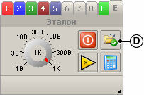
Analog Channel Tab

Logical channel tab

Reference channel tab

1. Tab of the currently active channel.
2. Tab of an inactive enabled channel.
3. An overline indicates that the channel data has been inverted.
4. Tab of the disabled channel.
5. Field for setting the name of the channel.
6. Channel on/off button. On – green background, off – red background.
7. Button for opening the window for mathematical processing of channel data (at the development stage).
8. Button to turn on / off the visual inversion of channel data.
9. Channel input range selection knob.
   1. Button with a drop-down menu for selecting a channel setting.
   2. Flag on / off the pulse detector at the input of the logical channel (LC).
   3. Field for setting the threshold value with which the amplitude of the LC input signal is compared.
   4. Button to call the dialog for opening the template file.

Keyboard Shortcuts:

Select the corresponding analog channel as the active channel:Ctrl+1…8 Select a logical channel as the active channel:ctrl+9 Select reference channel as active channel:ctrl+0

Enable / disable the corresponding analog channel:Alt+1…8 Enable/ disable logical channel:Alt+9 Show / hide reference channel graph:Alt+0

Note

At least one of the channels must be enabled.

Sweep panel

The sweep panel is designed to set the following sampling parameters: § sample rate/period, sample length,

§

§ pre-trigger length,

§ the length of the recorder window (the number of displayed readings at a scale of 1:1).

Oscilloscope mode,

synchronization

off

Oscilloscope mode,

synchronization

enabled

recorder mode,

synchronization

off

recorder mode,

synchronization

enabled

The maximum allowable sample rate is automatically adjusted when changing the registration mode and switching channels on / off. Invalid sample rates are shown in pale gray. Also, depending on the selected mode and the number of enabled channels, the maximum allowable values of the sample and pre-trigger lengths are automatically corrected. The pre-trigger length field is visible only when synchronization is enabled.

In the figure of the schematic representation of the measurement parameters, the blue line corresponds to the signal section before the synchronization moment, the red color line – after the synchronization moment. The green arrow indicates the type of synchronization used: unidirectional – absolute synchronization, bidirectional – differential synchronization. Synchronization on a logical channel is indicated by two straight horizontal lines with a corresponding transition (front).

Synchronization panel

The synchronization panel is designed to set the following synchronization parameters: § sync on/off, sync source channel selection,

§ sync edge selection,

§

§ select the type of synchronization to use,

§ setting the threshold difference between the amplitudes of neighboring readings.

• • • 1. Synchronization on / off button with a drop-down menu for selecting the synchronization source channel.
      2. Button for selecting the synchronization on the leading edge.
      3. Falling edge trigger selection button.
      4. Button for selecting the absolute type of synchronization.
      5. Button for selecting the differential type of synchronization.
      6. Schematic representation of synchronization conditions.
      7. Field for setting the threshold difference between the amplitudes of adjacent readings.

Enable synccan be done in the following ways: §

click the on button. / off locking it in the recessed state, select one of the synchronization source

§ channels (it will be enabled automatically), move the mouse wheel over the button to select one of the

§ synchronization source channels.

Turn off synccan be done in the following ways: §

click the on button. / off synchronization, unchecking it, in

§ the drop-down menu, select the item “Turn off”,

§ move the mouse wheel over the button until the “Disable” item is selected.

Forsync source channel selectionclick on the arrow in the lower right corner of the button. / off synchronization, or if the channel is not selected, then simply click on the button, and then select the desired channel in the pop-up menu that appears. Forshifts channeljust roll the mouse wheel over the button until the the name of the channel you are looking for in the button title.

The drop-down menu displays a list of only the channels currently on, i.e. if the desired channel is not in the list, then it must first be turned on.

On button / off Synchronization also allows you to inform about a long “absence” of synchronization. If after starting the registration process with the

synchronization, the specified synchronization conditions were not met within the time allotted for this, the button turns red, signaling a long “lack of” synchronization. If there is no synchronization for a long time, it is not necessary to manually stop the registration process, it is enough, if necessary, to simply change the synchronization conditions.

Advice

If, after starting the registration process, nothing appears on the screen for a long time, then it is possible that the synchronization conditions are waiting to be met, i.e. the device did not freeze.

Horizontal marker, which sets the level of absolute synchronization, will be visible only if the absolute synchronization type selection button is in the recessed state and one of the analog channels is selected as the synchronization source channel. The marker pointer is located near the axis of the synchronization source channel. In addition, the marker is automatically colored with the color of the synchronization source channel axis.

When moving the marker from the side opposite to the marker pointer, the current marker position (set level) will be displayed as a small hint. In addition, the current position will also be displayed in the status bar or marker tooltip.

Threshold difference setting field (absolute value of the difference between adjacent readings) will only be available if the differential sync type selection button is in the recessed state. If you enter an invalid value, the field frame will be colored red, informing you in advance that the specified synchronization condition cannot be met.

Marker Position Panel

The marker position panel is designed to display the values of the following values:

Equivalent frequency display

HF equivalent frequency display

1. The value of the current position on the time axis of the vertical marker 1.
2. The value of the current position on the time axis of the vertical marker 2.
3. The value of the length of the time interval between the positions of the vertical markers.
4. Equivalent to the length of the interval value of the frequency.
5. Equivalent to the length of the interval and the given angle, the value of the rotational speed of the CV.

Equivalent frequency value calculated from the expression: F = 1 / ∆T, i.e. specifies the number of intervals within 1 second. It is convenient to use the equivalent value of the frequency if it is necessary to calculate the repetition rate of certain sections of the signal. For example, to determine the PWM pulse repetition rate, it is necessary to place marker 1 at the beginning of one of the pulses, and marker 2 at the beginning of the next pulse, the resulting value of F corresponds to the desired pulse repetition rate.

Equivalent value of rotational speed KV calculated from the expression:

60 * (A / 360) / ∆T [rpm], where A is the specified angle of rotation of the crankshaft corresponding to the selected interval (the angle value is set in the settings window, on the “Oscilloscope” tab). It is convenient to use the equivalent value of the frequency of rotation of the CV if it is necessary to calculate the revolutions of the CV at which the studied section of the signal was obtained. For example, for the default value of the angle A = 720°, markers should indicate the signal section corresponding to the specified 720°, i.e. marker 1 must be placed at the beginning of one of the ignition pulses, and marker 2 at the beginning of the pulse going through the number of pulses equal to the number of cylinders.

If, for example, the angle is set to 720° / 4 = 180°, then for a 4-cylinder engine, the markers must indicate the signal section between adjacent ignition pulses, or if, for example, the markers indicate the section of one DPKV tooth (60 teeth), then the angle value should be 360° / 60 = 6°.

Summarizing the above, we formulate the procedure for semi-automatic determination of revolutions: 1. Determine the signal section with a predetermined length in the angles of rotation of the CV.

1. In the setting window, set a higher defined angle value.
2. Indicate with markers above a certain section of the signal.

To quickly change the displayed type of frequency, simply left-click on the heading / value of the frequency. And to quickly open the setup window with the “Oscilloscope” tab selected, just right-click on the heading / frequency value.

Control Panel

The control panel is intended for the following purposes: § selection of the registration mode, start / stop of the

§ registration process, display of the duration of the

§ registration process.

Panel view in oscilloscope mode

Panel view in frame mode or recorder

1. Oscilloscope mode acquisition selection button (F5).
2. Single frame registration selection button (F6).
3. Registration selection button in recorder mode (F7).
4. Button to start the registration process (F9) / stop the registration process (F11).
5. Button to start the registration process once (F9) / stop the registration process (F11).
6. The total duration of the registration process.

After starting the recording process, changing the mode directly in the recording process is only possible from the oscilloscope mode, which provides real-time configuration of the main parameters of the recording process and, if necessary, switching to the recording mode (by frame mode or recorder mode).

During registration in frame mode, it is possible to change almost all parameters, except for the number of enabled channels. During logging in recorder mode logging, changing any parameter of the logging process will not take effect until the next start, because after starting the instrument goes into continuous data transfer mode and does not respond to any commands. From which it follows that, for example, after starting in the recorder mode and the need to change the input range of any of the channels, it is initially necessary to stop the current registration process, then select the required range and then start the registration process again. At the same time, if there is no synchronization for a long time (button on / off synchronization is colored red), changes to the synchronization parameters will be automatically transferred both in frame-by-frame mode and in recorder mode, i.e. when changing synchronization settings, there is no need to manually stop the registration process.

For the frame-by-frame recording mode, the total recording duration takes into account only the duration of the samples of all recorded frames, without taking into account the delay time between frames.

Analog channel settings

Analog channel setting– a certain mathematical transformation of the measured voltage values into the value of the measured physical quantity corresponding to it. For example, a pressure sensor converts the measured pressure value into the corresponding voltage value, which in turn can be measured by an oscilloscope. The analog channel setting performs the inverse conversion, i.e. based on the value of the measured voltage, it calculates the corresponding pressure value, which makes it possible to display the pressure on the screen (the initial measured physical quantity).

To select an analog channel setting, click on the arrow in the lower right corner of the button with the drop- down menu for selecting the channel setting, and then select the required setting in the pop-up menu that appears by clicking on the menu item with its name. If there are no settings in the pop-up menu that appears, then you must first create them by opening the window for editing the list of settings.

After selecting the analog channel setup, the following controls and channel/axis parameters will be automatically configured (set):

§ The row of the channel input range selection knob will be recalculated in accordance with the specified boundaries of the measured physical quantity.

§ The axis limits will be recalculated to optimally display the signals within the given limits. The state of

§ the channel data inversion button will correspond to the relative position of the specified boundaries.

§ All dimensions of the channel data will correspond to the given dimension of the measured physical quantity.

If it is necessary to reconfigure, for example, after changing the axis boundaries or inverting the channel, it is enough just to click the left mouse button on the corresponding channel setup button, i.e. it is not necessary to reselect the current setting from the pop-up menu.

The window for editing the list of analog channel settings

To open the editing window, click on the arrow in the lower right corner of the channel settings button, and then select “Settings” in the pop-up menu that appears.

Note

To avoid tautology – analog channel setup, the term sensor is used in the editing window, which means the analog channel setup.

The window for editing the list of settings is intended for the following purposes: §

adding / deleting categories and sensors, correcting the display

§ order of categories and sensors, setting parameters for

§ categories and sensors,

§ opening / saving sensor parameters from / to a file.

Sensors are grouped into logically related groups – sensor categories, for example, secondary voltage sensors, pressure sensors, vacuum sensors or general purpose sensors. For simplicity, you can think of categories as folders and sensors as files stored in those folders. The sensor must necessarily belong to one of the existing categories, i.e. it is not possible to create a sensor without first creating / selecting the appropriate category.

The top part of the settings window is occupied by two lists: §

list of currently available categories, list of sensors

§ belonging to the selected category.

To add/remove list items, there are two corresponding buttons at the bottom of the lists. When a category is deleted, all sensors belonging to it are automatically deleted. Elements of both lists can be moved both with the mouse (select and drag) and with the help of the corresponding arrow buttons at the bottom of the lists. In addition, it is also possible to drag and drop sensors from the currently selected category to another category using the mouse.

The parameters of categories and sensors are displayed in the corresponding tabs occupying the main part of the settings window. The displayed parameters refer to the selected list item only, and when a category is selected, the Category Parameters tab automatically becomes active, and when a sensor is selected, the Sensor Parameters tab automatically becomes active. To select an element of the list, just left-click on its name.

Categories and sensors have several parameters of the same type: §

Name – designation of the category or sensor, corresponding to the title of the drop-down menu item of the analog channel setting selection button.

§ Description – brief information about the category or sensor displayed as a tooltip for the corresponding drop-down menu item.

§ Pictogram – a symbol of a category or sensor in the form of a picture (usually 24×24 px) displayed in the corresponding item of the drop-down menu.

§ The “Show” checkbox – allows / prohibits the display of the corresponding menu items. For example, it is convenient to temporarily hide rarely used sensors without deleting them.

In addition, the sensors have the following parameters: §

The category to which the sensor belongs.

§ Prefix – decimal prefix of the sensor value, for example Kilo (instead of 10,000 it will be 10K). The

§ dimension of the physical quantity measured by the sensor, for example, Pa, Atm, V, etc. Offset – the

§ value of the horizontal displacement of the sensor values along the time axis.

§ Transformation type – used mathematical transformation of the measured value.

Biassensor values along the time axis is mainly intended for visual sensor response time compensation. For example, some pressure sensors have a delay in changing the output voltage when the input pressure changes about 2 ms, which, when visually determining the ignition timing, can lead to an error equal to several tens of degrees. To reduce the error, it is necessary to set the offset equal to -2 ms, i.e. the graph will be shifted to the left by 2 ms, which will visually compensate for the delay introduced by the sensor.

The software of the MT Pro complex supports two types of conversion: §

limiting the boundaries of the input range of the channel by the boundaries of the measured physical

§ quantity, linear transformation of the measured voltage value into the corresponding value of the measured physical quantity.

Limitation it is convenient to use in the case of previously known limits of the signal under study. For example, the output voltage of an oxygen sensor is in the range of 0…1 Volt, which is much less than the maximum allowable ± 1000 Volt, from which it follows that it is possible to create an analog channel setting that limits the input range to 0…2 Volt. Using this setting will simply not allow a coarser channel input range to be selected, such as ±30V.

Linear transformation in addition to limiting the input range, allows you to set the ratio between the measured voltage value and the corresponding value of the measured physical quantity. Only relationships that satisfy the linear law (y = k⋅x + b), i.e. The scale of the sensor used must be linear. To set the ratio, it is necessary to set the boundaries of the measured physical quantity, and, based on the technical data of the sensor used, set the corresponding values of the measured voltage.

Let us illustrate the above with the example of a Honeywell MLH250PSB01A pressure sensor. Based on the technical data of the sensor, we determine: Minimum output voltage: 0.5 Volt Maximum output voltage:

4.5 Volt Sensor sensitivity: 0.235 Volt / Atm (linear dependence)

From which it follows that the output voltage of the sensor is determined based on the following relationship: U =

0.235 * P + 0.5 [Volt]

and the corresponding inverse transformation is as follows: P = (U – 0.5) / 0.235 [atm]

For simplicity, it is also possible to represent the above ratios in the form of a graph:

Since at speeds in the region of 1000 rpm only part of the pressure sensor scale is used, then, based on the recommendations for setting the boundaries of the control knob row, we will limit the scale from above to 10 atm. And taking into account a small vacuum in the cylinder, we continue the scale from the bottom to -1 Atm. Then, based on the above dependences or graph, we calculate the voltage values at the output of the pressure sensor corresponding to the selected pressure limits (measured physical quantity).

A pressure of -1 atm will correspond to an output voltage of 0.265 volts. A pressure of 10 atm will correspond to an output voltage of 2.855 volts.

Signal from a pressure sensor without using the analog channel setting

The same signal using tuning (all values in bar, ignition timing 17°)

There are several buttons at the bottom of the settings window: §

Open data file with sensor parameters. Save the

§ sensor parameters in the data file.

§ Restore – reset all changes made and restore the original information. OK – confirm all changes and close

§ the window.

§ Cancel – cancel all changes made and close the window.

Open buttonallows you to load the list structure, as well as the parameters of categories and sensors from an external data file (analogue channel settings database) received, for example, from other users.

Save buttonis designed to record the structure of the list, as well as the parameters of categories and sensors to the selected data file, which results in users sharing their analog channel settings.

Restore buttonperforms similar actions to the “Open” button, except that that the data will be automatically loaded from a file containing the initial list structure and default sensor parameters (set by the developers). When restoring, the current list and all sensor parameters will be lost, therefore, before restoring, if necessary, save the current list structure and sensor parameters in a separate file.

OK button confirms all changes made and closes the settings window. Everything changes made: adding / deleting categories or sensors, opening or restoring from a file, will not be visible in the oscilloscope window until the “OK” button is pressed.

Cancel button leads to the closing of the settings window without confirming all the entered changes,

i.e. the results of the actions taken will not take effect and will not be visible in the oscilloscope window.

Data about the list structure, sensor parameters and information about the selected analog channel settings are automatically saved in the following files when the application is terminated:

§ Sensors.sns is the main database that stores the list structure, as well as category and sensor parameters.

§ Sensors.bak is a backup copy of the database, if for some reason the main Sensors.sns file is damaged, then to restore the information, you must close the application and rename the Sensors.bak file to Sensors.sns.

§ Sensors.def is the default database used when clicking the “Restore” button. If necessary, this file can be updated by saving one of the versions of its own database. Sensors.cfg – data on the selected analog

§ channel settings. List of pointers (shortcuts) to the parameters of the selected setting of the corresponding analog channel.

Logical channel settings

A logical channel is functionally similar to an analog channel, except that the input signal is fed not to the ADC, but to a comparator with a comparison threshold configurable from the shell.

The output of the logical channel will correspond to a logical one if the value of the input voltage exceeds the set value of the comparison threshold, and to a logical zero if it does not.

The logical channel is convenient to use for synchronization and marking purposes, thereby “saving” the analog channel used for such purposes.

When synchronizing in oscilloscope mode and in frame mode, the logical channel is used as an external clock channel, the logical channel data is not displayed on the screen. When synchronizing in recorder mode, the capabilities of a logical channel are almost identical to those of analog channels. Also, in the recorder mode, the logical channel data is displayed on the screen in the same way as analog channels.

When marking the signal from the logical channel is used for unique identification during full working cycle, any characteristic section of the signal under study. For example, it is convenient to use a signal from a logical channel as a label for the first cylinder, in which case, theoretically, a single impulse of the logical channel during a complete operating cycle uniquely identifies the first cylinder.

To “improve” marking conditions from high-voltage wires,hardware detector impulses, which converts a narrow breakdown pulse into a wide “triangular” pulse. Usually, when using a logical channel as a label of the first cylinder, the threshold value is chosen equal to half the breakdown amplitude, while not taking into account two important factors:

§ the width of the markup pulse will be extremely narrow (several microseconds),

§ the presence of false impulses from sparking in neighboring cylinders (of the same width).

As can be seen from the figure, the breakdown voltage amplitude of the false pulse of the 3rd cylinder also exceeds the specified threshold value, which leads to the presence of two pulses at the output of the logical channel. Moreover, both pulses will be absolutely identical, since the width of the breakdown region of the true ignition pulse (1st cylinder) and the false ignition pulse (3rd cylinder) is the same.

From which it follows that in this case the basic principle of markup is not fulfilled – the presence of one unique label during the full work cycle, i.e. the program will not be able to determine which of the impulses is true.

The pulse detector converts the shape of the ignition pulse into a more convenient form for marking:

As can be seen from the figure, the pulse width at the output of the logical channel has increased significantly (several milliseconds). Although the false impulse of the 3rd cylinder still remains, but its width is much less than the width of the true impulse, which makes it possible for the program to uniquely identify the true impulse and perform further marking. The pulse detector automatically expands both negative and positive polarity pulses, which allows marking from any high-voltage DIS wire of ignition systems. In addition, having some internal threshold, the pulse detector automatically suppresses false pulses of small amplitude, in this case, the pulses of the 2nd cylinder are suppressed by the pulse detector.

Summarizing the above, we formulate the definition of the term logical channel setting. Setting up a logical channel– set of values of the following group of parameters: §

the selected input range of the logical channel, the threshold with

§ which the amplitude of the input signal is compared, the flag that

§ determines the state of the pulse detector.

The choice of the logical channel setting is carried out in the same way as the choice of the analog channel setting. After selecting a setting, the above group of parameters will be configured. For more efficient configuration, the corresponding logical channel settings elements are duplicated on the logical channel tab, which, if necessary, allows you to reconfigure without opening the settings window. Re-selection and reset of the setting is carried out in the same way as an analog channel, i.e. by clicking the channel setup button with the left or right mouse button.

Window for editing the list of logical channels settings

To open the editing window, click on the arrow in the lower right corner of the channel settings button, and then select “Settings” in the pop-up menu that appears.

The left part of the window is occupied by a list of available settings. All functions of interaction with the list (adding, deleting, moving, selecting) are similar to the corresponding functions from the window for editing the analog channel settings list. The main difference is the absence of categories, due to the small expected variety of logical channel settings.

The logical channel settings, as well as the analog channel settings, have the same general parameters: name, description, icon and the “Show” checkbox. The main settings (input range, threshold and pulse detector status flag) that directly affect the logical channel are located on the “Settings” panel.

The central part of the window is occupied by two screens displaying the shape of the analog signal at the input of the logical channel (working screen) and the graph of the crankshaft speed. On the right is the control panel containing the controls for the process of signal registration at the input of the logical channel.

Operating screen is designed to provide a visual setting of the parameters of the logical channel based on the shape of the input analog signal, i.e. tuning is performed on the basis of primary data, and not “blindly”. The signal at the input of the logical channel (before the comparator) is shown in the red graph, and the corresponding signal at the output of the comparator is shown in the blue graph.

• • • 1. The control axis of the analog signal graph.
      2. Graph of the analog signal at the input of the logical channel.
      3. Horizontal marker for visually setting

the value of the comparison threshold.

• • • 1. Graph of the corresponding logical signal at the output of the logical channel.
      2. Control axis of the logic signal graph.

The comparison threshold value can be set either directly through the “Threshold” field or using a horizontal marker, which is much more convenient for quick visual adjustment.

Control Panelis only intended to manage the registration process during visual setting of logical channel parameters. All adjustments related to the control panel do not affect these logical channel settings in any way.

The sample rate knob, as well as the sample length and pre-trigger length fields allow you to adjust the sample duration. For example, when analyzing the pulse width of the mark of the first cylinder (MPC), the optimal sample length is about 10 ms (combustion area + margin), and when controlling the specified parameters according to the graph of the CV speed at idle, the optimal sample length is at least 250 ms (2 [rev / mpc] / (600 [rpm] / 60 [sec])).

The sync enable checkbox and sync edge select buttons allow you to create the effect of a “stationary” signal when viewing, which is convenient when adjusting the parameters of the logical channel, since the pulse will be in the same location on the screen.

crankshaft speed chartdesigned for additional control given parameters of the logical channel used as the label of the first cylinder. The control is based on a visual check of the absence of sharp emissions on the graph with a smooth change in engine speed. Based on the fact that the mark of the first cylinder in the ideal case is a single impulse within the full working cycle, it follows that the crankshaft speed is determined as: 2 * 60 /∆T [rpm], where ∆T is the time interval between neighboring MOCs. When a false MOC appears, the calculated frequency value will increase by at least 2 times, since the interval between pulses will decrease, and if the MOC is skipped, the calculated frequency value will decrease by a maximum of 2 times, since the interval between pulses will increase.

As can be seen from the figure, a too low threshold value in the presence of high-amplitude false pulses leads to the appearance of false marks, i.e. in this case, to eliminate false labels, it is necessary to increase the threshold value. True labels are skipped because the threshold value is too high, which in this case must be reduced. The search for rare outliers allows you to quickly detect single false marks or single misses of true marks.

False label results in a jump up

Skipping a label results in a jump down

With a series of successive false marks or omissions, it is necessary to analyze directly the value of the CV revolutions. If 1200 rpm is displayed at idle instead of 600 rpm, i.e. every second mark is false (possibly an idle spark of the DIS system), then the threshold value must be increased. Or, with a sharp gas flow, the speed graph, instead of growing, drops sharply or stops being drawn at all, i.e. under load, the breakdown voltage drops significantly, then the threshold value must be reduced.

As the values of the horizontal axis of the graph, for definiteness, the conditional serial number of the time interval between adjacent MTCs is used (similar to the frame number). In the upper right corner, the revolutions calculated for the last time interval are displayed.

Note

To calculate the revolutions, at least two MOCs within one sample are required, for which it is enough to reduce the sampling frequency to 100 kHz, and increase the sample length to 30K.

At the bottom of the setup window there are the same buttons as in the analog channel setup window. The functionality of the buttons is the same.

List structure data, settings parameters and information about the selected logical channel settings are automatically saved in the following files when the application is terminated:

§ Slogics.slg is the main database. Slogics.bak is

§ a database backup. Slogics.def is the default

§ database.

§ Slogics.cfg – data about the selected logical channel settings.

Setting the logical channel as the label of the first cylinder

The mark of the first cylinder (MPC) is a single pulse within a complete working cycle that uniquely identifies the ignition pulse in the first cylinder. By unique identification is meant that the MOC is much closer to the ignition pulse in the first cylinder than to the pulses of the remaining cylinders. The start of the MOC does not have to coincide with the onset of breakdown in the first cylinder, the MOC just needs to be as close as possible to the ignition pulse in the first cylinder. Also, binding to the first cylinder is not obligatory, i.e. label, can identify any of the cylinders, since in most analysis algorithms both the number of the synchronization cylinder and the order of operation of the cylinders are specified.

Most often, in most diagnostic equipment, the signal from the high-voltage wire of the first cylinder is used as the source of the MPC. The MT Pro complex, having a universal logical channel, significantly expands the area of possible synchronization sources. So, for example, if it is not possible to obtain stable MOCs from signals from explosive wires, the following vehicle components can act as a source of MOCs:

§ primary ignition circuit,

§ injectors,

§ Hall Sensor,

§ DPKV,

§ pressure meter.

For example, we will give a sequence of actions for creating a logical channel setting, using the signal from the high-voltage wire of the first cylinder as a label for the first cylinder.

1. In the oscilloscope window, complete all current acquisition processes by clicking on the “Stop” button.
2. Open the window for editing the list of logical channels settings.
3. Create a new setting by clicking on the “Add” button.
4. Enter a name for the setting, for example “MPC”.
5. If necessary, open the corresponding icon.
6. Enable the pulse detector by checking the corresponding box.
7. Install the HV sensor on the HV wire of the 1st cylinder and connect it to the logic channel input.
8. Start the car engine.
9. Wait for the CV speed to be set corresponding to idling.
10. Select a sample rate of 200 kHz, set the sample length to 10K, and turn off the sync.
11. Start the registration process by clicking on the “Start” button.
12. Wait for the appearance of the signal graph at the input of the logical channel (a straight line is acceptable).
13. By reducing the input range of the channel, achieve the amplitude of the ignition pulses approximately equal to half the screen height of the working screen.
14. Set the threshold value to approximately half of the input range, and if the ignition pulses are directed

downwards, then the threshold value must also be negative.

1. Enable synchronization.
2. Verify that there is a wide (> 1 ms) stable pulse at the logic channel output.
3. If necessary, change the input range or adjust the level value to achieve a wide, stable sweep pulse.
4. Turn off synchronization.
5. Reduce sample rate to 100KHz, increase sample length to 30K.
6. Wait for the start of drawing the graph of the speed of the HF.
7. If the graph is not drawn, reduce the threshold value.
8. Verify that the displayed RPM is correct.
9. When displaying significantly overestimated revolutions – increase the threshold value, when displaying significantly lower revolutions – reduce the threshold value.
10. After pre-setting at idle, additionally check the stability of the formation of the MOC by increasing the speed of the CV to 2000 … 3000 rpm, as well as with a rapid increase in the speed, as a result of a short-term full opening of the throttle.
11. In the event of sharp spikes appearing on the HF speed graph, or if further drawing of the graph stops, try to change the input range or adjust the level value to achieve the stability of the MOC formation.
12. Stop the registration process by clicking on the “Stop” button.
13. Confirm the creation of the new setting and close the window by clicking on the “OK” button.

If by selecting the input range and adjusting the threshold value it was not possible to achieve a stable formation of the MOC, sharp spikes are observed on the CV speed graph, the displayed speed value is significantly overestimated or underestimated, it is recommended to perform the following actions:

§ change the location of the HV sensor on the HV wire,

§ move the HV sensor to the HV wire of another cylinder,

§ use the signal from the primary ignition circuit or injector as the source of the MPC.

If there is no stable formation of the MOC only under load, then when performing automatic diagnostics of the ignition system, it is advisable to start the diagnostics at idle, holding them for several seconds. Since it is quite possible that the analysis algorithm used will automatically take into account the presence of false or the absence of true marks, continuing the markup based on previously collected statistics at idle.

one hundred Copyright © 2009 www.mlab.org.ua

Work environment settings

Working environment– the totality of all application settings: § registration process parameters,

§ channel parameters, axes and graphs,

§ ruler parameters,

§ parameters of additional windows,

§ global application settings.

Saving a working environment in a settings file and then loading it from a settings file provides the ability to create a list of typical application settings. This saves a lot of time by setting up the application for a typical measurement once, then saving the settings and reloading them before starting the same typical measurement. For example, before diagnosing a DIS type ignition system, the application parameters are configured (channel parameters, sweep parameters, registration mode, etc. are set), after which the diagnostics are performed, after which the current settings are saved in the settings file. If, for example, after a few days, the diagnosis of the DIS ignition system needs to be carried out again,

It should also be noted that only links to the channel settings used are saved in the settings file, instead of saving the channel settings data directly (name, icon, etc.), which significantly reduces the volume of the settings file. From which it follows that when loading the working environment for the full configuration of the application, it is necessary to have all the analog and logical channel settings used in the working environment. When editing analog and logic channel setup lists, it is recommended that you do not delete channel setups that are used in saved workspaces.

To select a working environment, you must click on the arrow in the lower right corner of the button with a drop-down menu for selecting a working environment, or if the working environment has not yet been selected, then simply click on the button, after which in the appeared

pop-up menu to select the desired working

environment by clicking on the menu item with by his name. Also, the choice of the working environment can be done using only the keyboard, for

which you need to press the keyF12, then in the appeared pop-up menu using the keys , , , select the appropriate menu item and press the key Enter. Reselecting and resetting the work environment setup is done in the same way as channel setup, i.e. by clicking on the worker selection button with the left or right mouse button.

The window for editing the list of workspace settings

To open the editing window, click on the arrow in the lower right corner of the working environment selection button, and then select the “Settings” item in the menu that appears.

The top part of the settings window is occupied by the list of available categories and the list of workspace settings belonging to the selected category. All functions of interaction with the lists (adding, deleting, moving, selecting) are similar to the corresponding functions from the editing windows of the channel settings list.

Workspace settings, as well as channel settings, have the same general parameters: name, description, icon and the “Show” checkbox. The main parameter for setting the working environment is the name of the configuration file from which the working environment will be loaded when the corresponding menu item is selected, i.e. in fact, a workspace setup is just a link to the appropriate setup file. From which it follows that before starting to create a setting for the working environment, you must create the appropriate settings file, which actually contains all the settings.

To select a settings file, click on the […] button located at the end of the “Settings” field, and then in the dialog that opens, select the appropriate settings file. Also, the path to the file can be set directly in the “Settings” field. In addition, so-called relative paths are supported, i.e. the file path is relative to the base path to the application’s executable file. The use of relative paths allows, if necessary, to painlessly transfer the application to another folder or transfer the settings database to another user without subsequent adjustment of the paths to the settings files.

102 Copyright © 2009 www.mlab.org.ua

The “Default” pop-up menu item of the workspace selection button has a separate setting – an additional link to the default application settings file. This setting is no different from other settings, and the corresponding settings file must also be created beforehand. It is recommended to save the most frequently used application state (working environment) in the default settings file. The choice of the default settings file is carried out in the same way – by clicking on the […] button located at the end of the “Default” field, the ability to use a relative path is also supported for the default settings file.

Note

It is recommended to save the created settings files in the “Options \ WorkSpace” folder.

At the bottom of the settings window there are the same buttons as in the channels settings windows. The functionality of the buttons is the same.

Data about the structure of the lists, parameters of the settings of the working environment are automatically saved in the following files when the application is terminated:

§ WorkSpace.opt is the main database.

§ WorkSpace.bak is a database backup.

§ WorkSpace.def is the default database.

If you need to transfer the working environment settings database, please note that the settings are just links to the corresponding settings files, which in turn contain links to the channel settings used. From which it follows that with the working environment settings database, it is also necessary to transfer all settings files and channel settings databases.